Peihua Su
© 2022 IIETA. This article is published by IIETA and is licensed under the CC BY 4.0 license (http://creativecommons.org/licenses/by/4.0/).
OPEN ACCESS
In deep mines, thermal disasters pose a serious threat to the health and production efficiency of underground workers. It is of certain safety and economic significance to numerically simulate the thermal environment of hot mines. The existing studies are limited in that they only consider a single air flow velocity field or thermal field, or a single heat source. To overcome the limitation, this paper collects the big data on the temperature and humidity of smart coalmines, and numerically simulates the thermal environment in hot mines. Firstly, the authors analyzed the heat sources, including relative heat sources like the hot surrounding rock and hot water, and absolute heat sources like electromechanical equipment, chemical reactions, and the self-compression of the airflow. Next, the thermal environment of the hot mine was simulated by the Lattice Boltzmann method, and the flow state of the hot fluid in the roadways was analyzed in details. The proposed numerical simulation approach was proved effective through experiments, providing a reference for the safety prewarning of hot mines.
big data, hot mines, thermal environment, numerical simulation, safety prewarning
As coalmines go deeper into the ground, deep mine thermal disasters, a major constraint of mining safety, pose a serious threat to the health and production efficiency of underground workers [1, 2]. The high temperature of deep mines mainly comes from the great depth of the mines, the high fluidity of hot groundwater, and the small airflow on the mining face [3, 4]. What is worse, the water desorption of rocks, and the evaporation of mine water lead to a high humidity of deep mines, which magnifies the human and production damages of deep mine thermal disasters [5-8]. The big data on mine temperature and humidity can be collected by smart coalmines. If these data are fully utilized, it is possible to numerically simulate the thermal environment of hot mines, and contribute to the safety and economy of coalmining.
Based on internal heat sources, environment, and mine structure, Boubanga-Tombet et al. [9] created a hierarchical evaluation index system for the thermal environment of mines, and conducted a quantitative analysis of the thermal environment in the mines, using a neural network. To effectively monitoring the thermal environment of mines, Galkin [10] numerically simulated the thermal environment in the roadways of mines, with the aid of two models: uniform humidity model, and local humidity model. On this basis, the temperature and distribution of the surrounding rock were effectively predicted for mining operations. Lee [11] calculated thermal equilibrium parameters like skin temperature, skin humidity, sweating ratio, and working time limit of workers in underground mines, and concluded that the upper limit of the stope face temperature underground must fall between 27℃ and 28℃. Drawing on the concept of the thermal comfort zone, Hossain et al. [12] constructed a human thermal balance model, and divided the curve of the mean human skin temperature, which meets the thermal balance conditions of underground operators, into a working zone, a thermal comfort zone, and a non-working zone. Sasmito et al. [13] combined theoretical analysis with numerical simulation to estimate the thermal environment parameters of the mines, constructed a physical model and a mathematical model for examining the temperature distribution on the mining face and the change law of airflow enthalpy, and evaluated the air age and the predicted mean vote - predicted percentage of dissatisfied (PMV-PDD) index of the thermal environment in a mine. Gosiewski and Pawlaczyk [14] optimized support vector machine (SVM) with particle swarm optimization (PSO), and applied the optimized model to predict the thermal environmental parameters of the mine. Based on the calculated chilling requirement, they recommended the suitable power of air coolers for the mining face.
In summary, some studies on the thermal environment of hot mines merely consider a single air flow velocity field or thermal field. Hence, the simulated thermal environment disagrees with the actual situation [15-17]. Some only take account of a single heat source, failing to simulate the complex underground situation under the effect of multiple heat sources [18-22]. This paper collects the big data on the temperature and humidity of smart coalmines, and numerically simulates the thermal environment in hot mines. Section 2 analyzes the heat sources, including relative heat sources like the hot surrounding rock and hot water, and absolute heat sources like electromechanical equipment, chemical reactions, and the self-compression of the airflow. Section 3 numerically simulates the thermal environment of the hot mine by the Lattice Boltzmann method, analyzes the flow state of the hot fluid in the roadways, and expounds the relationship between air molecular movement and the complexity of underground airflow. The proposed numerical simulation approach was proved effective through experiments, providing a reference for the safety prewarning of hot mines.
The air temperature of mines is driven up by two kinds of heat sources: relative heat sources like the hot surrounding rock and hot water, and absolute heat sources like electromechanical equipment, chemical reactions, and the self-compression of the airflow. The ambient air temperature has a greater impact on the heat release of relative heat sources than on the heat release of absolute heat sources. Before numerically simulating the thermal environment of hot mines based on big data, this paper firstly analyzes and computes the possible heat sources and their heat release in general hot mines.
2.1 Relative heat sources
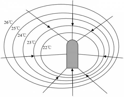
In the mine, the heat exchange between the surrounding rock and airflow is very complex, and rather uncertain. Figure 1 illustrates the heat transfer of the surrounding rock in a roadway. Let Ht be the heat release of the surrounding rock; C be the net section perimeter of the roadway; K be the length of the roadway; ψt be the mean original rock temperature at the two ends of the roadway; ψ be the mean temperature of the air flowing across the two ends of the roadway; Φt be the thermal conductivity of the rock, which determines the heat exchange coefficient between the surrounding rock and airflow. Then, the heat release of the surrounding rock can be calculated by:
$H_{t}=\Phi_{t} C K\left(\psi_{t}-\psi\right)$ (1)
For a roadway being ventilated for 1-10 years, Φt can be calculated by:
$\Phi_{t}=\frac{1}{1+\frac{\mu}{2 g E}}\left[\frac{\mu}{2 E}+\frac{f}{2 \sqrt{t}\left(1+\frac{\mu}{2 a E}\right)}\right]$ (2)
When the tunnel faces strong water evaporation, Φt can be calculated by:
$\Phi_{t}=\frac{\mu}{2 E}+\frac{f}{2 \sqrt{t}}$ (3)
Figure 1. Heat transfer of surrounding rock in a roadway
Let g be the convective heat release coefficient; gR be the heat release coefficient of the wet tunnel wall facing the airflow; μ be the thermal conductivity of the rock. For a roadway being ventilated for 1-10 years, we have:
$\Phi_{t}=\frac{\mu^{0.65} \quad (\sigma D)^{0.20} \quad g^{0.15}}{8.38 E^{0.45} \quad t^{0.20}}$ (4)
When the tunnel faces strong water evaporation, Φt can be calculated by:
$\Phi_{t}=\frac{\mu^{0.65} \quad (\sigma D)^{0.20} \quad g_{R}^{0.15}}{8.38 E^{0.45} \quad t^{0.20}}$ (5)
The g value can be approximated by:
$g=\frac{8.38 \delta Q^{0.8} C^{0.2}}{R}$ (6)
$f=8.39 \sqrt{\frac{\mu D \sigma}{\pi}}$ (7)
The gR value can be calculated by:
$g_{R}=g+9.75 \times 10^{-3} \beta$ (8)
The air flow and hot water exchange heat and water in the mine. The enthalpy difference is the main driver of the total heat exchange between them. This paper computes the total heat exchange amount H between hot water and the air, which is the sum between sensible heat exchange amount Ha and latent heat exchange amount Hk. Figure 2 illustrates the heat exchange between airflow and hot water. Let g be the heat exchange coefficient between the air and the surface of hot water; ψ be the ambient air temperature; ψf be the air temperature in the boundary layer; LH be the latent heat of vaporization of water; ε be the mass transfer coefficient between hot water and the air; MO be the moisture content of the air in the boundary layer; S be the contact area between the air and hot water. Then, we have:
Figure 2. Heat exchange between airflow and hot water
$H=H_{a}+H_{k}=\left[g\left(\psi-\psi_{h}\right)+L H \varepsilon\left(M O-M O_{h}\right)\right] S$ (9)
In the ventilation system of the mining area, the haulage roadway is treated as the intake airway. The local temperature rise in the roadway is mainly owed to the heat release of the coal and gangue being transported. Let n and ρn be the transport volume and specific heat of the coal and gangue being transported in the haulage roadway, respectively; Δψ be the temperature decrement of coal or gangue induced by cooling during the transport. Then, the heat release of the coal and gangue can be calculated by:
$H_{l}=n \rho_{n} \Delta \psi$ (10)
Let KTR be the transport distance; ψAV be the mean temperature of the coal and gangue being transported; ψSQ be the mean wet-bulb temperature of the airflow in the haulage roadway. Then, Δψ can be estimated by:
$\Delta \psi=0.0024 K_{T R}^{0.8}\left(\psi_{t}-\psi_{S Q}\right)$ (11)
2.2 Absolute heat sources
Under the action of gravity, the airflow moves downward along the mine. During the movement, the potential energy of the airflow is converted into heat, which increases the specific enthalpy. Figure 3 shows the enthalpy increase and heat release of the self-compression of the airflow. The heat of the airflow is imported to the mine as an external heat source. Let VD be the vertical depth increment of the mine. Then, the enthalpy increment Δj of the airflow induced by VD can be calculated by:
$\Delta j=9.81 \times V D \times 10^{-3}$ (12)
Let ρA be the specific heat of the air at constant pressure; Δψ be the increment of dry-bulb temperature of the airflow. Then, the enthalpy increment of the ideal gas satisfies Δj=ρAΔψ.
The heat release HSR of electromechanical equipment mainly includes frictional heat release and motor heat release. Let PA be the actual power consumption of the equipment; ξSR be the proportion of total power consumption used to increase the potential energy of mineral resources. Then, HSR can be calculated by:
$H_{S R}=P_{A}\left(1-\xi_{S R}\right)$ (13)
Figure 3. Enthalpy increase and heat release of the self-compression of the airflow
Let Δj be the enthalpy increment of the airflow after electromechanical equipment releases heat; QM be the mass flow of the airflow.
For underground substations, pump rooms, charging chambers, and electromechanically equipment chambers, the enthalpy increment of the airflow passing through each station/room/chamber can be derived from the humidity, temperature, and airflow measured at the inlet and outlet, as well as the psychrometric chart:
$H_{S R}=\Delta j \cdot Q_{M}$ (14)
For the heating of the airflow by local ventilators, the enthalpy increment of the airflow can be directly computed based on the input power of the motor. Let QM be the airflow mass of a local ventilator; AF be the airflow of the ventilator; WJ and WC be the static pressure and total pressure of the ventilator, respectively; ξJ and ξC be the total static pressure efficiency and total pressure efficiency of the ventilator, respectively; σ be the air density; PS be the input power of the motor. Then, the enthalpy increment of the airflow can be calculated by:
$\Delta j=\frac{P_{S}}{Q_{M}}=\frac{W_{J} \times 10^{-3}}{\sigma \xi_{J}}$ or $\Delta j=\frac{P_{S}}{Q_{M}}=\frac{W_{C} \times 10^{-3}}{\sigma \xi_{C}}$ (15)
where, PS can be calculated by:
$P_{S}=\frac{W_{J} \cdot A F \cdot 10^{-3}}{\xi_{J}}$ or $P_{S}=\frac{W_{C} \cdot A F \cdot 10^{-3}}{\xi_{C}}$ (16)
The temperature rise of the airflow passing through a local ventilator can be calculated by:
$\Delta \psi=\frac{\Delta j}{D_{O V}}$ (17)
Let HYW be the oxidative heat release; υ be the mean wind velocity in the tunnel; hYW be the heat release per unit area at υ=1m/s. Then, the oxidative heat release of underground minerals and other organics can be estimated by:
$H_{Y W}=h_{Y H} v^{0.8} C K$ (18)
As a reason of local temperature rise, the heat release by operators on the mining face play a nonnegligible role. Let mW be the total number of operators on the mining face; hR be the per-capita heat release. Then, the heat release of the operators Hpe can be calculated by:
$H_{p e}=m_{W} h_{R}$ (19)
The heat release from other heat sources is so small as to be negligible, such as trackless diesel engines, rock layer movement, auxiliary operations, and pressure ventilation pipes.
2.3 Thermal conductivity parameters
Reliable thermal conductivity of rocks and coal layer must be obtained to support the big data-based numerical simulation of the thermal environment of hot mines. This requires accurate analysis and computing of the thermal conductivity parameters of coal-bearing strata, as well as the heat release intensity of the surrounding rock induced by the rising ground temperature.
Let μ be the thermal conductivity of the coal sample; ωC and ωK be the upper layer temperature and lower layer temperature, respectively; ΔωC and ΔωK be the temperature difference in the upper part and the lower part, respectively; ΔωN be the temperature difference between the upper and lower surfaces of the coal sample; U be the thickness of the coal sample; UC and UK be the thickness of the overlying and underlying layers of the coal sample, respectively. By steady-state plate method, the specific heat flow SHF of the coal sample can be calculated by:
$S H F=\frac{\Delta \omega_{N}}{U}$ (20)
The SHF of the coal sample can also be calculated by comparing the upper and lower parts:
$S H F=\mu^{*}\left(\frac{\Delta \omega_{C}}{d_{C}}+\frac{\Delta \omega_{K}}{d_{K}}\right) / 2$
$\mu=g \Psi^{-1}+f$ (21)
If formula (20) equals formula (21), then:
$\mu=\frac{\mu^{*} U}{2 \Delta \omega_{N}}\left(\frac{\Delta \omega_{C}}{U_{C}}+\frac{\Delta \omega_{K}}{U_{K}}\right)$ (22)
The thermal conductivity of the rock sample can be measured by DRM-1 thermal conductivity detector. If the temperature in parts of the rock sample change cyclically, the time-variation rate of temperature in another part TD can be calculated. Let ρCPQ be the mass heat capacity of the rock sample at constant pressure; σRS be the density of the test block. Based on the TD value, the thermal conductivity of the rock sample can be further derived:
$\mu=10^{6} \mathrm{TD} \bullet \rho_{C P Q} \bullet \sigma_{R S}$ (23)
This section numerically simulates the flow law of the underground hot fluid by making full use of the big data on the temperature and humidity of various heat sources and the surrounding airflow, which are collected by well temperature and humidity transducers.
Currently, the flow of underground hot fluid is mainly investigated through numerical simulation. To clearly depict the relationship between air molecular movement and the complexity of underground airflow, this paper numerically simulates the thermal environment of the mine by the Lattice Boltzmann method, and solves the complex boundary problem.
The thermal environment of the mine was simulated by D2Q9 Lattice Boltzmann model. Let v be the migration velocity of air particles; Δa be the grid step length; Δτ be the time step length. The dispersion velocity vi in the nine directions of the model can be calculated by:
$v_{0}=(0,0)$
$v_{i}=\left(\cos \omega_{i}, \sin \omega_{i}\right) v,\left(\omega_{i}(i-1) \frac{\pi}{2}, i=1,2,3,4\right)$
$v_{i}=\sqrt{2}\left(\cos \omega_{i}, \sin \omega_{i}\right) v,\left(\omega_{i}(i-5) \frac{\pi}{2}+\frac{\pi}{4}, i=5,6,7,8\right)$
$v=\frac{\Delta a}{\Delta \tau}$ (24)
Let ε, σ, and β be model parameters; MA, and CO be the macro velocity and pressure of the air fluid, respectively. During the simulation of the thermal environment in the mine, the steady-state distribution function of internal energy can be adopted:
$q_{i}^{(E S)}=\left\{\begin{array}{l}-\frac{2}{3} \sigma \cdot r \cdot(M A \cdot M A), i=0 \\ \frac{1}{9} \sigma \cdot r\left[\frac{3}{2}+\frac{3}{2}\left(v_{i} \cdot M A\right)+\frac{9}{2}\left(v_{i} \cdot M A\right)^{2}-\frac{3}{2}(M A \cdot M A)\right] \\ i=1,2,3,4\\\ \frac{1}{36} \sigma \cdot r\left[3+6\left(v_{i} \cdot M A\right)+\frac{9}{2}\left(v_{i} \cdot M A\right)^{2}-\frac{3}{2}(M A \cdot M A)\right] \\ i=5,6,7,8\end{array}\right.$ (25)
The steady-state density distribution function can also be adopted:
$q_{i}^{(E S)}=\left\{\begin{array}{l}-\frac{4 \varepsilon \sigma}{v^{2}}-\frac{2 M A^{2}}{3 v^{2}}, i=0 \\ \frac{\alpha \sigma}{v^{2}}+\frac{v_{i} \cdot M A}{3 v^{2}}+\frac{\left(v_{i} \cdot M A\right)^{2}}{2 v^{4}}-\frac{M A^{2}}{6 v^{2}}, \quad i=1,2,3,4 \\ \frac{\beta \cdot C O}{v^{2}}+\frac{v_{i} \cdot M A}{12 v^{2}}+\frac{\left(v_{i} \cdot M A\right)^{2}}{8 v^{4}}-\frac{M A^{2}}{24 v^{2}}, i=5,6,7,8\end{array}\right.$ (26)
MA can be calculated by:
$M A=\sum_{i} v_{i} q_{i}, C O=\frac{v^{2}}{4 \varepsilon}\left[\sum_{i} q_{i}+\frac{4}{9}\left(-1.5 \frac{M A^{2}}{C O^{2}}\right)\right]$ (27)
Let ΨM=Σ4i=1Ψi be the macro temperature of the air fluid. Then, the steady-state distribution function of temperature can be established as:
$\Psi_{i}^{(E S)}=\frac{\Psi}{4}\left[1+2 \frac{v_{i} \cdot M A}{v_{i}^{2}}\right], i=1,2,3,4$ (28)
The complex underground roadway was numerically simulated through decomposition-coupling and TD2G9 model. The dispersion velocity of the model can be calculated by:
$\left\{\begin{array}{l}(0,0) \quad i=0 \\ (\cos [(i-1) \pi / 2], \sin [(i-1) \pi / 2]) v \quad i=1,2,3,4 \\ \sqrt{2}(\cos [(i-5) \pi / 2+\pi / 4], \sin [(i-5) \pi / 2+\pi / 4]) v \\ i=5,6,7,8\end{array}\right.$ (29)
The evolution of the model can be described as:
$\Psi_{i}\left(a+v_{i} \Delta \psi, \psi+\Delta \psi\right)-\Psi_{i}(a, \psi)$
$=-\frac{1}{t_{\Lambda}}\left[\Psi_{i}(a, \psi)-\Psi_{i}^{E S}(a, \psi)\right] \quad i=1 \sim 4$ (30)
The macro velocity, pressure, and temperature of the air fluid can be respectively calculated by:
$M A=\sum_{i=1}^{8} v_{i} q_{i}$ (31)
$C O=\frac{v^{2}}{4 \varepsilon}\left[\sum_{i=1}^{8} q_{i}+H G_{0}(M A)\right]$ (32)
$\Psi=\sum_{i=1}^{4} v_{i} q_{i}$ (33)
The viscosity coefficient and heat diffusion coefficient of air turbulence can be respectively calculated by:
$F R=\frac{1}{3}\left(t_{M 4}-\frac{1}{2}\right) \frac{\Delta a^{2}}{\Delta \psi}$ (34)
$H E=\left(t_{\Psi}-\frac{1}{2}\right) \frac{\Delta a^{2}}{\Delta \psi}$ (35)
Six temperature measuring points were selected on a mining face in a mine. The elevation from point P1 to P6 gradually increases. Table 1 lists the temperature measured at these points. Along the airflow direction, the temperature at P2, which has a low elevation, was higher than that at the other points. By contrast, the temperature at P1, which has a high elevation, was relatively low. This is because P1 is close to the inlet of the intake airway, so that the airflow exchanges heat with the surrounding rock only for a short period before reaching this point.
The target mining face has a 1,350m-long intake airway. Thermal disasters are severe in the study area, due to heat release by hot surrounding rock and hot water. The highest temperature was observed at the junction between the end of the intake airway and the mining face, and the lowest was observed at the air intake. Taking the middle of the roadway as the origin, the direction pointing to the surface was defined as the negative direction. A temperature measuring point was set up at an interval of 100m from the origin to both sides. In total, 21 points were deployed from -1,000m to 1,000m. Table 2 shows the measured temperatures. Judging by temperature distribution, the temperature of the mining face was already above 28℃, failing to meet the safety standard of mines. The main reason is the sustained heat release from the surrounding rock to the airflow, as well as the heat release from electromechanical equipment.
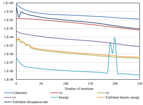
The lattice file of the thermal environment of the mine was solved by Fluent3D solver. Firstly, the minimum volume of the grids was determined as positive, and the segregated-implicit algorithm was selected to solve the steady-state flow. Since heat transfer is involved the thermal environment of the mine, the energy equation must be activated. Then, the law of underground air fluid was simulated by the turbulent model, which solves the turbulent kinetic energy, turbulent dissipation rate, and turbulent viscosity. Based on the Boussinesq assumption for natural convection, the Reynolds stress was solved accurately.
The iterative computing was carried out after setting the material properties of the fluid, boundary conditions, and number of iterations. To deeply understand the model convergence through numerical simulation, the convergence of each parameter was monitored by a residual curve monitor. In addition, this paper deploys a monitor for the mean temperature of outlet cross-section to judge if the temperature at each monitoring point reaches the ideal steady state, and to capture the exact variation of roadway outlet temperature. Figures 4 and 5 present the curves of convergence residuals, and the variation of the mean temperature of outlet cross-section, respectively.
Table 1. Temperatures measured at different points
|
Measuring point |
Surface temperature |
P1 |
P2 |
P3 |
P4 |
P5 |
P6 |
|
Elevation/m |
-550 |
-500 |
-500 |
-400 |
-350 |
-300 |
|
|
1 |
15℃ |
17℃ |
30℃ |
30℃ |
24℃ |
21℃ |
23℃ |
|
2 |
22℃ |
20℃ |
31℃ |
31℃ |
26℃ |
24℃ |
25℃ |
|
3 |
27℃ |
18℃ |
28℃ |
29℃ |
25℃ |
23℃ |
26℃ |
|
4 |
26℃ |
19℃ |
32℃ |
32℃ |
27℃ |
22℃ |
27℃ |
|
5 |
25℃ |
17℃ |
33℃ |
34℃ |
26℃ |
25℃ |
28℃ |
|
6 |
27℃ |
16℃ |
29℃ |
33℃ |
29℃ |
27℃ |
26℃ |
|
7 |
28℃ |
15℃ |
31℃ |
35℃ |
30℃ |
26℃ |
27℃ |
|
8 |
28℃ |
18℃ |
35℃ |
31℃ |
28℃ |
25℃ |
28℃ |
|
9 |
30℃ |
19℃ |
32℃ |
32℃ |
27℃ |
23℃ |
25℃ |
|
10 |
25℃ |
21℃ |
34℃ |
34℃ |
25℃ |
25℃ |
28℃ |
Table 2. Distribution of measured temperature in the intake airway
|
-1000 |
900 |
-800 |
-700 |
-600 |
-500 |
-400 |
-300 |
-200 |
-100 |
0 |
|
17 |
18 |
19 |
20 |
21 |
22 |
23 |
22 |
24 |
26 |
27 |
|
100 |
200 |
300 |
400 |
500 |
600 |
700 |
800 |
900 |
1000 |
|
|
28 |
29 |
29 |
30 |
31 |
31 |
31 |
30 |
30 |
30 |
|
Figure 4. Convergence residual curve
Figure 5. Curve of the variation of mean temperature of outlet cross-section
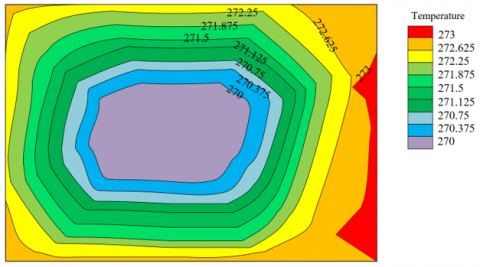
Figure 6. Temperature distribution of the outlet cross-section at 0m
Figure 7. Temperature distribution of the outlet cross-section at 200m
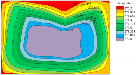
Figure 8. Temperature distribution of the outlet cross-section at 400m
Figure 9. Temperature distribution of the outlet cross-section at 600m
Figure 10. Roadway temperature variation
Figures 6-9 display the simulated temperature distribution of the outlet cross-section at different positions. Along the airflow direction, the roadway and wall became hotter and hotter, owing to the heat exchange between the surrounding rock and the airflow. The temperature peaked at 29.45℃, as the airflow reached 800m.
The airflow temperature is not very different from the surrounding rock temperature in actual underground roadways. There is already a stable heat regulation circle. Therefore, the simulated temperature at the center of the roadway and its change trend were close to the actual situation at each measuring point in the intake airway. Figure 10 presents the curve of roadway temperature variation. Table 3 lists the simulated temperature at each point in the intake airway.
Figure 11 compares the simulated temperature at each point with the real-time measured value. It can be seen that the simulated values at most points were slightly greater than the measured values. The main reason is the neglection of the real-time air humidity measured by humidity sensors. In the actual roadway, the humidity is as high as 0.6-0.9. The temperature rise of the roadway mainly stems from the latent heat of vaporization and heat exchange, both of which are caused by the wall rock temperature. If the air humidity is introduced, the calculation would be closer to the actual situation, and provide a reference for real-time safety prewarning of hot mines.
Table 3. Simulated temperature at each point in the intake airway
|
-1000 |
900 |
-800 |
-700 |
-600 |
-500 |
-400 |
-300 |
-200 |
-100 |
0 |
|
17.24 |
18.35 |
19.21 |
20.37 |
21.16 |
21.54 |
22.32 |
22.89 |
23.06 |
24.25 |
25.68 |
|
100 |
200 |
300 |
400 |
500 |
600 |
700 |
800 |
900 |
1000 |
|
|
27.71 |
29.52 |
28.03 |
29.94 |
29.35 |
30.76 |
30.18 |
30.87 |
29.26 |
30.71 |
|
Figure 11. Measured temperature vs. simulated temperature at each measuring point
Figure 12. Roadway temperature variation at different wind velocities
Figure 13. Roadway tunnel curves at different inlet air velocities and temperatures
Figure 12 shows the roadway temperature variation at different wind velocities. The change rate of roadway temperature is represented by the slope corresponding to the tangent line at each point on the curve. It can be seen that, along the airflow direction, the temperature rise gradually slowed down. With the growing heat exchange between the airflow and the surrounding rock, the curve approximated a straight line. In this case, it is impossible to reduce the roadway temperature to the safety threshold by increasing ventilation alone. Figure 13 present the tunnel temperature curves at different temperatures and velocities of inlet air. The slope of the tunnel temperature curve gradually increased, and the temperature increment of the roadway became more prominent, with the decline of temperature, and growth of velocity. This is mainly due to the fact that the temperature is negatively correlated with heat exchange velocity, and roadway temperature increment. Increasing air velocity or lowering air velocity alone cannot effectively cool down the roadway. It is necessary to consider both inlet air velocities and temperatures at the same time.
Based on the big data on the temperature and humidity of mines, this paper numerically simulates the thermal environment of hot mines. After analyzing both relative and absolute heat sources, the authors simulated the thermal environment of hot mines by Lattice Boltzmann method, and analyzed the flow state of the hot fluid in the roadways. Then, the lattice file of the thermal environment of the mine was solved by Fluent3D solver. Through simulation, the curves of convergence residuals, and the variation of the mean temperature of outlet cross-section were plotted. The curves show that the simulated temperature at the center of the roadway and its change trend were close to the actual situation at each measuring point in the intake airway, providing a reference for real-time safety prewarning of hot mines. Finally, the roadway tunnel curves were drawn at different inlet air velocities and temperatures. The results show that a good cooling effect cannot be achieved unless both inlet air velocities and temperatures are considered at the same time.
This paper was supported by the Shaanxi Provincial Department of Science and Technology Industrial Public Relations Project "Research on monitoring mechanism of tailings dam deformation based on wireless sensor network location" (Grant No.: 2018GY-095).
[1] Boulanger-Martel, V., Bussière, B., Côté, J. (2021). Thermal behaviour and performance of two field experimental insulation covers to control sulfide oxidation at Meadowbank mine, Nunavut. Canadian Geotechnical Journal, 58(3): 427-440. https://doi.org/10.1139/cgj-2019-0616
[2] Lan, B., Li, Y.R. (2018). Numerical study on thermal oxidation of lean coal mine methane in a thermal flow-reversal reactor. Chemical Engineering Journal, 351: 922-929. https://doi.org/10.1016/j.cej.2018.06.153
[3] Chu, Z., Zhou, G., Bi, S. (2018). Meso-characterization of the effective thermal conductivity of selected typical geomaterials in an underground coal mine. Energy Exploration & Exploitation, 36(3): 488-508. https://doi.org/10.1177%2F0144598717740956
[4] Galhardi, J.A., García-Tenorio, R., Francés, I.D., Bonotto, D.M., Marcelli, M.P. (2017). Natural radionuclides in lichens, mosses and ferns in a thermal power plant and in an adjacent coal mine area in southern Brazil. Journal of Environmental Radioactivity, 167: 43-53. https://doi.org/10.1016/j.jenvrad.2016.11.009
[5] Taylor, K., Banks, D., Watson, I. (2016). Heat as a natural, low-cost tracer in mine water systems: The attenuation and retardation of thermal signals in a Reducing and Alkalinity Producing Treatment System (RAPS). International Journal of Coal Geology, 164: 48-57. https://doi.org/10.1016/j.coal.2016.03.013
[6] Burnside, N.M., Banks, D., Boyce, A.J. (2016). Sustainability of thermal energy production at the flooded mine workings of the former Caphouse Colliery, Yorkshire, United Kingdom. International Journal of Coal Geology, 164: 85-91. https://doi.org/10.1016/j.coal.2016.03.006
[7] Ding, J., Zhang, P. (2015). Coupled 3D fluid field & thermal field calculation of mine-used explosion-proof integrative variable-frequency motor. Electric Machines and Control, 19(7): 27-35. https://doi.org/10.15938/j.emc.2015.07.005
[8] Philippe, G., Abdoulaye, G., Haïkel, B.H., Hassen, B., Farid, L. (2019). Installation of a thermal energy storage site in an abandoned mine in Picardy (France). Part 1: Selection criteria and equipment of the experimental site. Environmental Earth Sciences, 78(5): 174. https://doi.org/10.1007/s12665-019-8128-0
[9] Boubanga-Tombet, S., Huot, A., et al. (2018). Thermal infrared hyperspectral imaging for mineralogy mapping of a mine face. Remote Sensing, 10(10): 1518. https://doi.org/10.3390/rs10101518
[10] Galkin, A.F. (2015). Efficiency evaluation of thermal insulation use in criolithic zone mine openings. Metallurgical and Mining Industry, 7(10): 234-237.
[11] Lee, J.K., Shang, J.Q., Jeong, S. (2015). Thermal conductivity of compacted fill with mine tailings and recycled tire particles. Soils and Foundations, 55(6): 1454-1465. https://doi.org/10.1016/j.sandf.2015.10.010
[12] Hossain, M., Paul, S.K., Hasan, M. (2015). Environmental impacts of coal mine and thermal power plant to the surroundings of Barapukuria, Dinajpur, Bangladesh. Environmental Monitoring and Assessment, 187(4): 202. https://doi.org/10.1007/s10661-015-4435-4
[13] Sasmito, A.P., Kurnia, J.C., Birgersson, E., Mujumdar, A.S. (2015). Computational evaluation of thermal management strategies in an underground mine. Applied Thermal Engineering, 90: 1144-1150. https://doi.org/10.1016/j.applthermaleng.2015.01.062
[14] Gosiewski, K., Pawlaczyk, A. (2014). Catalytic or thermal reversed flow combustion of coal mine ventilation air methane: What is better choice and when? Chemical Engineering Journal, 238: 78-85. https://doi.org/10.1016/j.cej.2013.07.039
[15] Lee, J.K., Shang, J.Q. (2014). Evolution of thermal and mechanical properties of mine tailings and fly ash mixtures during curing period. Canadian Geotechnical Journal, 51(5): 570-582. https://doi.org/10.1139/cgj-2012-0232
[16] Yantek, D.S., Yan, L., Damiano, N.W., Reyes, M.A., Srednicki, J.R. (2019). A test method for evaluating the thermal environment of underground coal mine refuge alternatives. International Journal of Mining Science and Technology, 29(3): 343-355. https://doi.org/10.1016/j.ijmst.2019.01.004
[17] Moukannaa, S., Nazari, A., Bagheri, A., Loutou, M., Sanjayan, J.G., Hakkou, R. (2019). Alkaline fused phosphate mine tailings for geopolymer mortar synthesis: Thermal stability, mechanical and microstructural properties. Journal of Non-Crystalline Solids, 511: 76-85. https://doi.org/10.1016/j.jnoncrysol.2018.12.031
[18] Kaya, S., Leloglu, U.M. (2017). Buried and surface mine detection from thermal image time series. IEEE Journal of Selected Topics in Applied Earth Observations and Remote Sensing, 10(10): 4544-4552. https://doi.org/10.1109/JSTARS.2016.2639037
[19] Ghoreishi-Madiseh, S.A., Sasmito, A.P., Hassani, F.P., Amiri, L. (2017). Performance evaluation of large scale rock-pit seasonal thermal energy storage for application in underground mine ventilation. Applied Energy, 185: 1940-1947. https://doi.org/10.1016/j.apenergy.2016.01.062
[20] Karamahmut Mermer, N., Sari Yilmaz, M., Dere Ozdemir, O., Piskin, M.B. (2017). The synthesis of silica-based aerogel from gold mine waste for thermal insulation. Journal of Thermal Analysis and Calorimetry, 129(3): 1807-1812. https://doi.org/10.1007/s10973-017-6371-8
[21] Sari Yilmaz, M., Acaroglu Degitz, I., Piskin, S. (2017). Thermal analysis applied for the removal of surfactant from mesoporous molecular sieves MCM-41 synthesized from gold mine tailings slurry. Journal of Thermal Analysis and Calorimetry, 130(2): 727-734. https://doi.org/10.1007/s10973-017-6490-2
[22] Ranjan, S., Das, D.C., Sinha, N., Latif, A., Hussain, S.S., Ustun, T.S. (2021). Voltage stability assessment of isolated hybrid dish-stirling solar thermal-diesel microgrid with STATCOM using mine blast algorithm. Electric Power Systems Research, 196: 107239. https://doi.org/10.1016/j.epsr.2021.107239