Shefali Jauhri* | Upendra Mishra
© 2021 IIETA. This article is published by IIETA and is licensed under the CC BY 4.0 license (http://creativecommons.org/licenses/by/4.0/).
OPEN ACCESS
In this paper stagnation boundary layer flow of nanofluid with mixed convection heat and mass transfer with Electrical Magneto Hydrodynamic (EMHD) effects over a second-order momentum slip boundary condition have been mathematically analysed. The governing equations are transformed by similarity variable and the problem becomes coupled third-order nonlinear coupled differential equations. We use fourth-order Runge Kuta method and shooting technique to find the solution. The effect of second-order momentum slip condition with linear thermal slip condition has determined. Variation of all nano energy conversion parameters depends on different factors has shown graphically. Some of the parameters possesses dual solution at different values of second-order velocity slip parameter $\left(\beta_{1} \& \beta_{2}\right)$.
EMHD, nano-fluid, similarity transformation, Runge Kutta method, dual solution
The study of viscous incompressible fluid over a slip stretching sheet with stagnation fluid problem occurring in several engineering processes such as atomic reactor cooling, cooling of an enormous metallic plate, polymer expulsion, drawing of copper wires, paper creation, hot moving, wire drawing, glass-fiber, metal expulsion has increased significantly. These applications with second-order slip condition are very helpful in the solution of flow problems because using of continuum description as compared to molecular-based approaches. Ongoing progression in present-day innovation has intrigued the consideration of specialists toward the investigation of warmth move marvels. Along these lines, the examination of heat transfer in different basic circumstances has increased because of their important utility in vitality creation, atomic reactor cooling, cooling of an enormous metallic plate in a shower, in polymer expulsion, drawing of copper wires, counterfeit strands, paper creation, hot moving, wire drawing, glass fiber, metal expulsion and metal turning applications, and so on. In this paper, our point is centered around the impact of second-order slip velocity boundary on stagnation flow over a stretching-sheet with mixed convection heat and mass transfer with electrical magneto hydrodynamics, which has not been examined before. We discuss that increasing the values of second-order momentum slip parameters $\beta_{1} \& \beta_{2}$ & electric parameter E with linear thermal slip parameter we get dual solution for temperature profile. Also, we show that the impact of free convection parameters $G_{t}$ at the thermal flow procedure brings out the inverse effect of temperature.
Ahmed [1] worked on Walters Liquid B Model, boundary layer flow over a stretching plate. He solved heat transfer problem with variable thermal conductivity in two different parts, first one is the prescribed surface temperature and second one is the prescribed stretching plate heat flux. Ahmed [2] Discussed the boundary layer flow of viscous incompressible fluid over a stretching plate. He explained the effect of suction parameter with variable thermal conductivity on temperature field in two different parts, first one is the prescribed surface temperature and second one is the prescribed stretching plate heat flux. Anderson [3] researched the viscoelastic fluid on a stretching surface in the presence of a transverse magnetic field and obtained the exact analytic solution of the boundary layer very.
Bachok et al. [4] investigated the time independent 2D stagnation point flow of nanofluid on a stretching/shrinking sheet and the velocity he assumed is vary with distance from stagnation point. Bentwhich [5] investigate the semi-infinite assortment of viscous incompressible fluid problem. He considered a two-dimensional semi-infinite stream and acquired the solution of low Reynold number with stokes Oseen solution. Chen [6] discussed the laminar boundary layer flow on a linearly stretching sheet. He considered two cases first the sheet with prescribed wall temperature and the second is heat flux on a continuous surface. Chiam [7] explained the solution of the energy equation for the boundary layer flow of an electrically conducting fluid under the influence of a constant transverse magnetic field over a linearly stretching non-isothermal flat sheet.
Choi et al. [8] was the person who uses nanofluids and demonstrated that the expansion of a modest quantity (under 1% by volume) of nanoparticles to regular warmth move fluids expanded the thermal conductivity of the liquid up to around multiple times. Crane [9] was the first one who discovered the exact solution of heat transfer on the linear stretching sheet. Dash et al. [10] considered the magnetohydrodynamics stream, warmth, and mass dispersion of an electrically directing zero velocity point stream over an extending/contracting sheet considering the synthetic response of diffusing species and inside warmth generation/absorption. The oddity of the current examination is two-overlap: (I) to dissect the warmth move angle (ii) to talk about the effect of resistive electromagnetic power on the stream wonders.
Fang and Aziz [11] acquired a diagnostic arrangement of the MHD stream along with a contracting sheet with the main request slipstream. Fang et al. [12] investigated the slipstream over a penetrable contracting surface with the recently proposed Wu's slip speed model. Fang et al. [13] discussed the magnetohydrodynamic (MHD) stream under slip condition over a porous extending surface is understood systematically. The arrangement is given in a closed structure condition and is a definite arrangement of the full overseeing Navier–Stokes conditions. The impacts of the slip, the magnetic, and the mass exchange boundaries are discussed.
Hayat [14] discuss the aspects of buoyancy force on second-order magnetic viscous nano-fluid and the effect of different parameters like Brownian-motion, viscous dissipation, and thermophoresis viewpoints are presented in the detailing of the issue. Hsiao [15] explained the transformation issues of conjugate conduction, convection, and radiation warmth, and mass exchange with thick scattering and attractive impacts have been explored. Hsiao [16] discussed the magnetohydrodynamic (MHD) stream under slip condition over a porous extending surface is understood systematically. The arrangement is given in a closed structure condition and is a definite arrangement of the full overseeing Navier Stokes conditions. The impacts of the slip, the magnetic, and the mass exchange boundaries are discussed.
Hsiao [17] investigated the stagnation nano energy conversion problem with a mixed convection boundary value problem. Ishak [18] considered the warmth move over an extending surface with variable warmth motion in micropolar liquids. Ishak et al. [19] the heat transfer over a temperamental extending surface with recommended divider temperature has been discussed. Junoh et al. [20] research the consistent magnetohydrodynamics (MHD) limit layer zero speed point stream of an incompressible, thick, and electrically leading liquid past an expanding/contracting sheet with the effect of incited magnetic field.
Kang et al. [21] numerically and exploratory investigated nanofluids cover heat conductivity. Khanafer et al. [22] analyzed the heat transfer execution of nanofluids inside a closed-in area taking into account the strong molecule scattering. After these creators, nanotechnology is considered by numerous individuals to be one of the critical powers that drive the following major mechanical transformation of this century. It speaks to the most important mechanical front line right now being investigated. It targets controlling the structure of the issue at the sub-atomic level with the objective for development in for all intents and purposes each industry and open undertaking including organic sciences, physical sciences, hardware cooling, transportation, the earth, and national security etc. Khan & Pop [23] numerically investigated the laminar fluid flow problem over a flat surface on a stretching sheet of nanofluid.
Kumaran and Ramanaiah [24] worked on viscous incompressible flow over a stretching sheet. The velocity he considered in his paper is a quadratic polynomial of the distance from the slit and the sheet is subjected to a linear mass flux. Kuznetsov & Nield [25] examined the regular convective boundary layer flow of a nanofluid past a vertical plate analytically. Furthermore, clarify the impacts of Brownian movement and thermophoresis. Malavandi et al. [26] investigated nanoparticle of different type on stretching/shrinking sheet with stagnation point flow. Merkin and Pop [27] the impact that a stagnation-point stream on an extending/contracting surface can have on an exothermic surface response is considered. The velocity of the surface comparative with the external stream is estimated by the boundary parameter (λ) with there being a basic estimation.
Mishra and Singh [28] examined the ‘Axisymmetric’ stream of a viscous incompressible liquid over a contracting vertical surface with the thermal flow is examined considered the second-order momentum slip and first-order heat slip boundary condition. Mishra and Singh [29] explained the boundary layer stream and heat transfer of an incompressible liquid along a vertical temperamental extending sheet in a peaceful liquid is introduced on the off chance that when temperature distinction among sheet and encompassing liquid. Myers et al. [30] has demonstrated the effect of the different parameters of heat & mass transfer on nanofluid experimentally.
Nadeem et al. [31] numerically investigated the heat transfer of Maxwell fluid on stretching sheet. Ramesh et al. [32] consistent 2D boundary layer stream of a thick dusty fluid over a stretching sheet with the base surface of the sheet warmed by convection from a hot liquid. Reddy et al. [33] investigated thermal effect with radiation & magnetic field over an inclined vertical plate. Siddappa and Abel [34] investigated the crane’s flow problem to the visco-elastic fluid of Walter's liquid model and obtained the solution of the equation of motion for boundary layer flow past a stretching sheet. Subhas and Veena [35] discussed the visco-elastic fluid flow and heat transfer characteristics in a saturated porous medium over an impermeable stretching surface with frictional heating and heat generation or absorption. He considered PHF (Prescribed Heat Flux) & PST (Prescribed Surface Temperature) cases and obtained the solution for the velocity field and skin friction. Wang [36] researched the extension of crane’s paper. He worked on the three-dimensional fluid motion on a flat boundary stretching sheet and find the exact solution of Navier Stokes's condition.
The Boundary-Layer with slip condition on stretching surface is now an important part of research and the stagnation point flow problem pulling the attention of numerous specialists for over a century in view of its wide applications. In this paper we considered the time independent 2D boundary layer flow of an incompressible nano fluid stretching surface under a second order velocity slip boundary condition with variable thermal conductivity. The stream is thought to be in the x-direction, which is brought the slightly upward way furthermore, y-direction is in normal direction. The considered fluid equations are taken from Hasio [16] are as follows,
$\frac{\partial u}{\partial x}+\frac{\partial v}{\partial y}=0$ (1)
$\begin{aligned} u \frac{\partial u}{\partial x}+v \frac{\partial u}{\partial y}=u_{\infty} & \frac{\partial u_{\infty}}{\partial x}+v_{f} \frac{\partial^{2} u}{\partial y^{2}}+\sigma \frac{B_{0}^{2}}{\rho_{f}}(U-u) \\ &+g_{x} \beta_{t}\left(T-T_{\infty}\right)+g_{x} \beta_{c}\left(C-C_{\infty}\right) \\ &+\sigma \frac{E_{0} B_{0}}{\rho_{f}} \end{aligned}$ (2)
$\begin{aligned} u \frac{\partial T}{\partial x}+v \frac{\partial T}{\partial y}=& \frac{K_{f}}{\left(\rho c_{p}\right)_{f}} \frac{\partial^{2} T}{\partial y^{2}}+\frac{Q_{0}}{\left(\rho c_{p}\right)_{f}}\left(T-T_{\infty}\right) \\ &+\frac{\left(\rho c_{p}\right)_{p}}{\left(\rho c_{p}\right)_{f}}\left[D_{B} \frac{\partial C}{\partial y} \frac{\partial T}{\partial y}+\frac{D_{T}}{T_{\infty}}\left(\frac{\partial T}{\partial y}\right)^{2}\right] \end{aligned}$ (3)
$u \frac{\partial C}{\partial x}+v \frac{\partial C}{\partial y}=D_{B} \frac{\partial^{2} C}{\partial y^{2}}+\frac{D_{T}}{T_{\infty}} \frac{\partial^{2} T}{\partial y^{2}}$ (4)
In Eq. (2) the term $u_{\infty} \frac{\partial u_{\infty}}{\partial x}$ is stagnation point flow with $\theta=90^{\circ}$ in $u_{\infty} \frac{\partial u_{\infty}}{\partial x} \sin \theta . \cdot B_{0}$ is defining the variable magnetic factor, while $E_{0}$ electric field parameter, $g_{x}$ is gravity-magnitude and ‘T’ is fluid-temperature. $G_{t} \& G_{c}$ are thermal free and mass free convection parameter and explaining the mixed convection effect. $v_{f}$ is kinematic-viscosity, $\beta_{t} \& \beta_{c}$ are thermal expansion and mass diffusion. Similarly other terms of Eqns. (3) & (4) are define in nomenclature. The following equations are described on electrical magnetics flow field. Here ‘u’ is the velocity-component heading to x-axis i.e., along the surface and v is in y direction i.e., normal to it. Here assumed thermal conductivity $k_{f}$ is variable thermal conductivity and defined as $k_{f}=k_{\infty}(1+\varepsilon \theta)$ (by Ahmed [1]), where $\varepsilon=\frac{k_{f}-k_{\infty}}{k_{\infty}}$.
Subject to the boundary conditions are,
$\left.\begin{array}{c}\mathrm{u}=\mathrm{Cx}+L_{1} v \frac{\partial u}{\partial y}+L_{2} v \frac{\partial^{2} u}{\partial y^{2}}, v=0 \\ \mathrm{~T}=T_{W}+k_{1} \frac{\partial T}{\partial y} \\ C=C_{W}+k_{2} \frac{\partial C}{\partial y}\end{array}\right\}$ at $y=0$ (5)
$\left.\begin{array}{c}u \rightarrow 0 \\ T \rightarrow T_{\infty} \\ C \rightarrow C_{\infty}\end{array}\right\}$ as $y \rightarrow \infty \quad x_{1,2}=\frac{-b \pm \sqrt{b^{2}-4 a c}}{2 a}$ (6)
Here $L_{1}$ and $L_{2}$ are slip parameter in reference of velocity and v is the kinematic-viscosity and ‘C’ is the proportionality constant. Here $k_{1}$ is slip parameter in reference of temperature. Here $k_{2}$ is slip parameter in reference of concentration.
Similarity variables are:
$\eta=y \sqrt{\frac{a}{v_{f}}}$
$u=a x f^{\prime}(\eta)$ and $v=-\sqrt{a v_{f}} f(\eta)$ (7)
Defining the non-dimensional temperature and concentration variable are:
$\theta(\eta)=\frac{T-T_{\infty}}{T_{W}-T_{\infty},}, \phi(\eta)=\frac{C-C_{\infty}}{C_{W}-C_{\infty}}$
$\mathrm{T}=T_{\infty}+A x \theta(\eta)$ and $\mathrm{C}=C_{\infty}+B x \phi(\eta)$ (8)
Using Eqns. (8) and (9) in Eqns. (2), (3) & (4). The transformed DE. are,
$f^{\prime \prime \prime}+f f^{\prime \prime}-f^{\prime 2}+M\left(1-f^{\prime}\right)+G_{t} \theta+G_{c} \phi-M E=0$ (9)
$\theta^{\prime \prime}+\operatorname{Pr}\left[f \theta^{\prime}+\lambda \theta+N_{b} \theta^{\prime} \phi^{\prime}+N_{t} \theta^{\prime 2}\right]+\varepsilon\left(\theta \theta^{\prime \prime}+\theta^{\prime 2}\right)=0$ (10)
$\phi^{\prime \prime}+\operatorname{Sc} f \phi^{\prime}+\frac{N_{t}}{N_{b}} \theta^{\prime \prime}=0$ (11)
The boundary conditions are:
$\left.\begin{array}{c}f=0, f^{\prime}=1+\beta_{1} f^{\prime \prime}+\beta_{2} f^{\prime \prime \prime} \\ \theta(0)=1+\delta_{1} \theta^{\prime}(0) \\ \phi(0)=1+\delta_{2} \phi^{\prime}(0)\end{array}\right\}$ at $\eta=0$ (12)
$\left.\begin{array}{rl}f^{\prime} & \rightarrow 0 \\ \theta & \rightarrow 0 \\ \phi & \rightarrow 0\end{array}\right\}$ as $\eta \rightarrow \infty$ (13)
where, $\beta_{1}=L_{1} \sqrt{a v}$ and $\beta_{2}=a L_{2}$, are called second and third order coefficient of slip parameter. $\delta_{1}=K_{1} \sqrt{\frac{a}{v}}$ and $\delta_{2}=K_{2} \sqrt{\frac{a}{v}}$ are called thermal slip coefficient and mass diffusion slip coefficient. According to Ahmed [1] the transfer of heat done by two parts, one is due to temperature difference and the other one is due to variable thermal conductivity. In Eq. (10), the term independent of $\varepsilon, i . e \theta^{\prime \prime}+\operatorname{Pr}\left[f \theta^{\prime}+\lambda \theta+N_{b} \theta^{\prime} \phi^{\prime}+N_{t} \theta^{\prime 2}\right]=0$ is due to temperature difference and the second part i.e., $\left(\theta \theta^{\prime \prime}+\theta^{\prime 2}\right)$=0 is due to variable thermal conductivity.
SKIN FRICTION: Skin friction is resistance to flow of fluid over the surface, influenced by surface roughness and velocity of the fluid and defined as,
$C_{f}=\left.\frac{\tau}{\frac{1}{2} \rho u^{2}}\right|_{y=0}$
where, $\tau$ is shear stress and defined as, $\tau=\mu \frac{\partial u}{\partial y}$.
Hence,
$C_{f}=\left.\frac{\mu \frac{\partial u}{\partial y}}{\frac{1}{2} \rho u^{2}}\right|_{y=0}=\frac{2 f^{\prime \prime}(0)}{\sqrt{R e}}$
Therefore, the skin friction coefficient:
$f^{\prime \prime}(0)=\frac{1}{2} \sqrt{\operatorname{Re}} C_{f}$
2.1 Nusselt number
If there should arise an occurrence of conduction, the heat transfer can be determined utilizing Fourier's law of conduction. If there should arise an occurrence of convection, the heat transfer can be determined by Newton's law of cooling. The Nusselt number explain the difference of heat transfer through a liquid layer because of convection comparative with conduction over a similar fluid layer. The Nusselt number can be defined as,
$N u=\frac{x q_{w}}{k_{f}\left(T_{w}-T_{\infty}\right)}$
2.2 Sherwood number
Sherwood number is used in mass transfer activity. Additionally, it is called as Nusselt number in mass transfer. It speaks to the proportion of the convective mass exchange to the rate of diffusive mass transport. The Sherwood number can be defined as,
$S h=\frac{x q_{m}}{D_{B}\left(C_{w}-C_{\infty}\right)}$
Here,
$q_{w}$=heat flux.
$q_{m}$=mass flux.
k=coefficient of thermal conductivity.
x=characteristic length.
By using Eq. (9) we get,
$\frac{N u}{R e_{x}^{1 / 2}}=-\left[1+\frac{\varepsilon \theta(0)}{1+\varepsilon \theta(0)}\right] \theta^{\prime}(0), \frac{S h}{R e_{x}^{1 / 2}}=-\phi^{\prime}(0)$.
where, $R e_{x}=\frac{u_{w} x}{v}$ is known as local Reynolds number.
In this paper the system we have considered is heat conduction-convection system and the system of equations we have considered are highly non-linear PDE. So, to find exact solution is highly complexed. We use similarity variable to convert non-linear PDE into non-linear ODE. Fourth order Runge–Kutta technique along with shooting strategy has been utilized to examine the model. The impact of second order slip parameter is discussed in Eqns. (9)-(11) in the presence of various parameters like Prandtl number Pr, Magnetic-parameter ‘M’, Electric-parameter ‘E’, a Brownian movement parameter ‘Nb’, a thermophoresis parameter ‘Nb’, Schmidt number ‘Sc’. We used RK4 to solve the system of equations with shooting strategy. We introduced the following new variable to convert the system of nonlinear differential equation into first order ODE.
$f_{1}=f, f_{2}=f^{\prime}, f_{3}=f^{\prime \prime}, f_{4}=\theta, f_{5}=\theta^{\prime}, f_{6}=\phi, f_{7}=\phi^{\prime}$
And the Eqns. (9)-(11) becomes,
$f_{1}^{\prime}=f_{2}, f_{2}^{\prime}=f_{3}$ (14)
$f_{3}^{\prime}=-f_{1} * f_{3}+f_{2}^{2}-M\left(1-f_{2}\right)-G_{t} f_{4}-G_{c} f_{6}+\mathrm{ME}$ (15)
$f_{4}^{\prime}=f_{5}$ (16)
$f_{5}^{\prime}=-\varepsilon\left(f_{4} * f_{5}^{\prime}+f_{5}^{2}\right)-\operatorname{Pr} *\left[f_{1} * f_{5}+\lambda * f_{4}+\right.$
$\left.N_{b} f_{5} * f_{7}+N_{t} * f_{5}^{2}\right]$ (17)
$f_{6}^{\prime}=f_{7}$ (18)
$f_{7}^{\prime}=-S c f_{1} f_{7}+\frac{N_{t}}{N_{b}} f_{5}^{\prime}$ (19)
With boundary conditions,
$f=0, f_{2}=1+\beta_{1} f_{3}+\beta_{2} f_{3}^{\prime} \quad$ at $\eta=0$ (20)
$\begin{aligned} f_{2} & \rightarrow 0 \text { as } \eta \rightarrow \infty \\ f_{4}(0) &=1+\delta_{1} f_{5}(0), \phi(0)=1+\delta_{2} f_{7}(0) \\ f_{4} & \rightarrow 0 \text { as } \eta \rightarrow \infty, f_{6} \rightarrow 0 \text { as } \eta \rightarrow \infty \end{aligned}$ (21)
After that we applied Runge Kutta method along with shooting method to find numerical solution.
In Table 1 we have shown the comparison of present result of $-\theta^{\prime}(0)$ and $-\phi^{\prime}(0)$ with the result of khan & Pop [22] for various physical parameters $N_{t} \& N_{b}$ and the other constant parameters $G_{t}=G_{c}=\lambda=\mathrm{M}=\mathrm{E}=\delta=\delta_{1}=\delta_{2}=\mathrm{S}=0$ and Sc = Pr = 10.
Table 1. Comparison of the result with Khan and Pop [23]
|
$N_{t}$ |
$N_{b}$ |
$-\theta^{\prime}(0)$ Khan &Pop |
$-\theta^{\prime}(0)$ Present Result |
$-\phi^{\prime}(\mathbf{0})$ Khan &Pop |
$-\phi^{\prime}(\mathbf{0})$ Present Result |
|
0.1 |
0.1 |
0.9524 |
0.952375 |
2.1294 |
2.129384 |
|
0.2 |
0.2 |
0.3654 |
0.365362 |
2.5152 |
2.515210 |
|
0.3 |
0.3 |
0.1355 |
0.135489 |
2.6088 |
2.608799 |
|
0.4 |
0.4 |
0.0495 |
0.049543 |
2.6038 |
2.603786 |
|
0.5 |
0.5 |
0.0179 |
0.017921 |
2.5731 |
2.573121 |
The changed momentum, temperature and concentration Eqns. (9)-(11) with boundary conditions Eqns. (12) & (13) were numerically solved by utilizing Runge–Kutta fourth order strategy alongside shooting method. We acquired velocity, temperature profile graph for various benefits of overseeing parameters. The mixed convection issue related with time independent, non-linear, two-dimensional stagnation point nanofluid flow over a stretching surface is altogether examined & numerical outcomes are obtained. The BLP defined is changed into an IVP by shooting strategy. As the analytic strategies flop to understand the arrangement of different conditions together. The outcomes acquired are shown through Figures 1-7 for temperature, velocity & concentration profile respectively.
Figure 1. The physical model for stagnation mixed convection flows with EMHD and heat effects of incompressible nanofluid over a stretching sheet
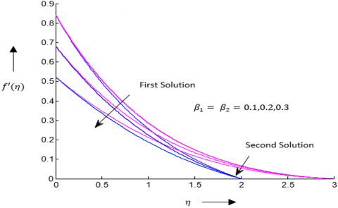
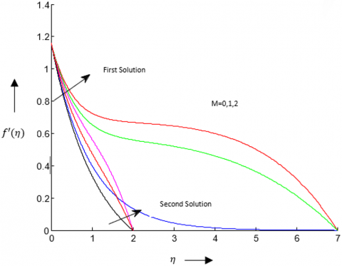
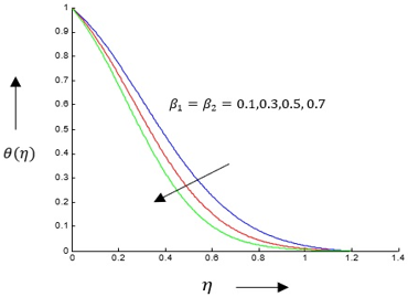
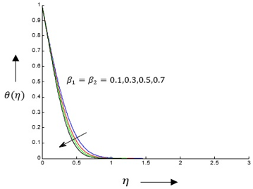
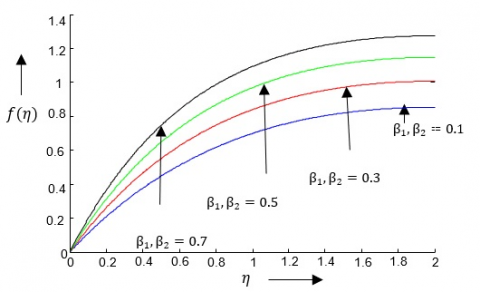
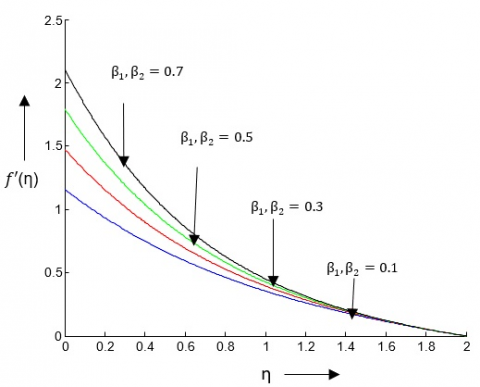
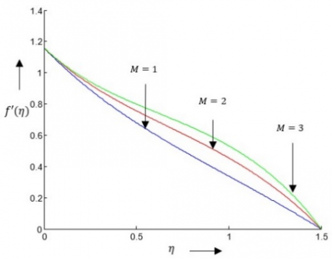
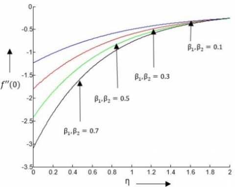
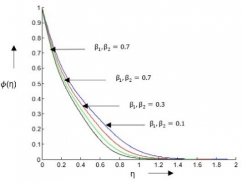
We can analyse that velocity profile showing dual solution on different values of second order slip parameters $\beta_{1} \& \beta_{2}$, in Figure 2(a) and for magnetic parameter in Figure 2(b). Figure 3(a) and 3(b) representing dual solution of temperature profile on different values of second order slip parameters $\beta_{1} \& \beta_{2}$. In Figure 5(a), 5(b), 6(b) & 7(a) we found that on increasing the value of $\beta_{1} \& \beta_{2}$, stream function, momentum, skin friction & mass transfer all reduced.
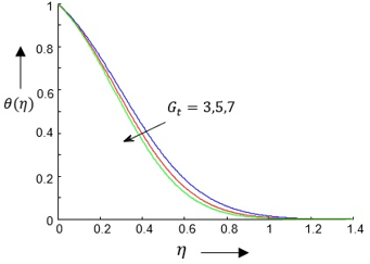
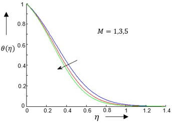
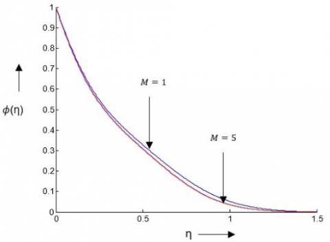
Figure (4(b), 6(a) &7(b) are graph of temperature, velocity & mass transfer on different values magnetic parameter and we can see that as ‘m’ increases, temperature, velocity & mass transfer decreases. In Figure 4(a) we can analyse that as ‘$G_{t}$’ increases temperature decreases.
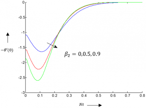
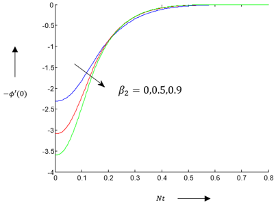
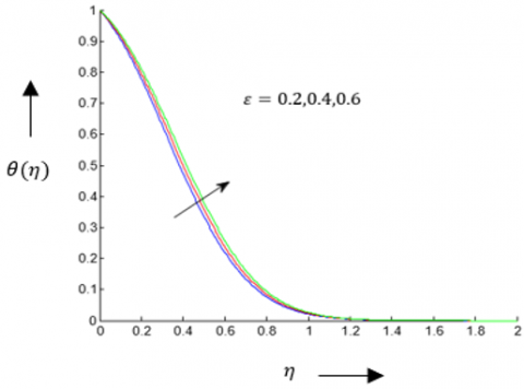
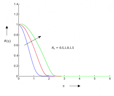
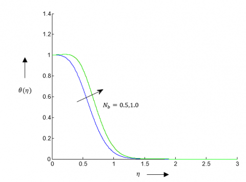
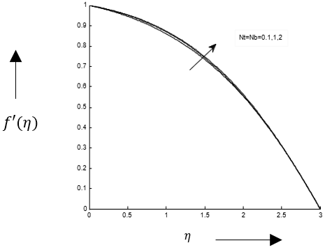
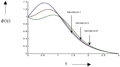
Figure 8(a) & 8(b) are graph of Nusselt Number & Sherwood Number at different values of second order slip parameters $\beta_{2}$. In both graph we are getting node and both are decreasing. In Figure 9 it is identified that increasing the value of $\varepsilon$, temperature profile decreases. Figures 10(a) & 10(b) are temperature profiles & Figures 10 (c) & 10(d) are velocity & mass diffusion profile for different values of $N_{t}, N_{b}$. It is identified that increasing the values of $N_{t}, N_{b}$ temperature and velocity profile are increasing while mass transfer is decreasing.
(a)
(b)
Figure 2. (a) is representation of dual solution of velocity profiles for different values of $\beta_{1} \& \beta_{2}$ versus $\eta$ & (b) is representation of dual solution of velocity profiles for different values of M versus $\eta$ with $E=0.1, N t=0.1, N b=0.1, \lambda=0.1, G t=0.1, G c=0.1, P r=10, S c=10, \varepsilon=0$
(a)
(b)
Figure 3. (a & b) are temperature profiles for different values of $\beta_{1} \& \beta_{2}$ versus $\eta$ with $M=0.1, E=0.1, N t=0.1, N b=0.1, \lambda=0.1, G t=0.1, G c=0.1, P r=10, S c=10, \varepsilon=0$
(a)
(b)
Figure 4. (a) & (b) are temperature profiles for different values of m versus $\eta \& G_{t}$ versus $\eta$ for $\beta_{1}=\beta_{2}=0.1$ when $E=0.1, N t=0.1, N b=0.1, \lambda=0.1, G c=0.1, P r=10, S c=10, \varepsilon=0$
(a)
(b)
Figure 5. (a) & (b) is stream function profiles & velocity profiles for different values of $\beta_{1}, \beta_{2}$ versus $\eta$ when $E=0.1, N t=0.1, N b=0.1, \lambda=0.1, G c=0.1, P r=10, S c=10, \varepsilon=0$
(a)
(b)
Figure 6. (a) & (b) are velocity profiles & skin friction profiles for different values of m versus $\eta \& \beta_{1}, \beta_{2}$ versus $\eta$ when $E=0.1, N t=0.1, N b=0.1, \lambda=0.1, G c=0.1, P r=10, S c=10, \varepsilon=0$
(a)
(b)
Figure 7. (a) & (b) are mass diffusion profiles for different values of $\beta_{1}, \beta_{2}$ versus $\eta$ & M versus $\eta$ when $E=0.1, N t=0.1, N b=0.1, \lambda=0.1, G c=0.1, P r=10, S c=10, \varepsilon=0$
(a)
(b)
Figure 8. (a) & (b) are Nusselt Number & Sherwood Number profiles for different values of $\beta_{1}=0.1, \beta_{2}$ versus $N_{t}$ when $M=0.1, E=0.1, N t=0.1, N b=0.1, \lambda=0.1, G c=0.1, \operatorname{Pr}=10, S c=10, \varepsilon=0$
Figure 9. Temperature profiles for different values of versus $\varepsilon$ when $M=0.1, E=0.1, N t=0.1, N b=0.1, \lambda=0.1, G c=0.1, P r=10, S c=10$
(a)
(b)
(c)
(d)
Figure 10. (a & b) are temperature profiles & (c & d) are velocity & mass diffusion profile for different values of $N_{t}, N_{b}$ versus $\eta$ when $M=0.1, E=0.1, N t=0.1, N b=0.1, \lambda=0.1, G c=0.1, \operatorname{Pr}=10, S c=10, \varepsilon=0.1$
To test the stability of the dual solutions. We consider the unsteady form of Eq. [(2-4) in paper)] with boundary conditions (5) & (6) as,
$\begin{aligned} \frac{\partial u}{\partial t}+u \frac{\partial u}{\partial x}+v \frac{\partial u}{\partial y} & \\=& u_{\infty} \frac{\partial u_{\infty}}{\partial x}+v_{f} \frac{\partial^{2} u}{\partial y^{2}} \\ &+\sigma \frac{B_{0}^{2}}{\rho_{f}}(U-u)+g_{x} \beta_{t}\left(T-T_{\infty}\right) \\ &+g_{x} \beta_{c}\left(C-C_{\infty}\right)+\sigma \frac{E_{0} B_{0}}{\rho_{f}} \end{aligned}$ (22)
$\begin{aligned} \frac{\partial T}{\partial t}+u \frac{\partial T}{\partial x}+v \frac{\partial T}{\partial y} & \\=& \frac{K_{f}}{\left(\rho c_{p}\right)_{f}} \frac{\partial^{2} T}{\partial y^{2}}+\frac{Q_{0}}{\left(\rho c_{p}\right)_{f}}\left(T-T_{\infty}\right) \\ &+\frac{\left(\rho c_{p}\right)_{p}}{\left(\rho c_{p}\right)_{f}}\left[D_{B} \frac{\partial C}{\partial y} \frac{\partial T}{\partial y}+\frac{D_{T}}{T_{\infty}}\left(\frac{\partial T}{\partial y}\right)^{2}\right] \end{aligned}$ (23)
$\frac{\partial C}{\partial t}+u \frac{\partial C}{\partial x}+v \frac{\partial C}{\partial y}=D_{B} \frac{\partial^{2} C}{\partial y^{2}}+\frac{D_{T}}{T_{\infty}} \frac{\partial^{2} T}{\partial y^{2}}$ (24)
Subject to the boundary conditions are,
$\left.\begin{array}{c}\mathrm{u}=\mathrm{Cx}+L_{1} v \frac{\partial u}{\partial y}+L_{2} v \frac{\partial^{2} u}{\partial y^{2}}, v=0 \\ \mathrm{~T}=T_{W}+k_{1} \frac{\partial T}{\partial y} \\ C=C_{W}+k_{2} \frac{\partial c}{\partial y}\end{array}\right\}$ at $y=0$ (25)
$\left.\begin{array}{c}u \rightarrow 0 \\ T \rightarrow T_{\infty} \\ C \rightarrow C_{\infty}\end{array}\right\}$ as $y \rightarrow \infty$ (26)
Using similarity transformations equations become,
$f^{\prime \prime \prime}+f f^{\prime \prime}-f^{\prime 2}+M\left(1-f^{\prime}\right)+G_{t} \theta+G_{c} \phi-$
$\mathrm{ME}+f_{t}^{\prime}=0$ (27)
$\frac{1}{P r} \theta^{\prime \prime}+f \theta^{\prime}+\lambda \theta+N_{b} \theta^{\prime} \phi^{\prime}+N_{t} \theta^{\prime 2}+\theta_{t}^{\prime}=0$ (28)
$\phi^{\prime \prime}+S c f \phi^{\prime}+\frac{N_{t}}{N_{b}} \theta^{\prime \prime}+\phi_{t}^{\prime}=0$ (29)
The boundary conditions are,
$\left.\begin{array}{c}f=0, f^{\prime}=1+\beta_{1} f^{\prime \prime}+\beta_{2} f^{\prime \prime \prime} \\ \theta(0)=1+\delta_{1} \theta^{\prime}(0) \\ \phi(0)=1+\delta_{2} \phi^{\prime}(0)\end{array}\right\}$ at $\eta=0$ (30)
Here $f, \theta, \phi$ are of function of $(\eta, t)$.
Stability of the dual solutions are determined by adopting the stability analysis of Merkin [37] we put,
$\left.\begin{array}{rl}f(\eta, t) & =f_{0}(\eta)+e^{-\gamma t} F(\eta, t) \\ \theta(\eta, t) & =\theta_{0}(\eta)+e^{-\gamma t} T(\eta, t) \\ \phi(\eta, t) & =\phi_{0}(\eta)+e^{-\gamma t} C(\eta, t)\end{array}\right\}$ (31)
where, $\gamma$ is unknown eigen values and $f_{0}, \theta_{0}, \phi_{0}$ satisfy steady boundary condition. Here $F(\eta, t), T(\eta, t), C(\eta, t)$ and all its derivatives are assumed small compared with the steady solution $F(\eta)$ and its derivatives. Because we are studying the linear stability analysis.
Hence our Unsteady equations become,
$F_{0}^{\prime \prime \prime}+F_{0} f_{0}^{\prime \prime}+f_{0} F_{0}^{\prime \prime}-F_{0}^{2}-2 F_{0} f_{0}-M F_{0}^{\prime}+T_{0} G_{t}$
$+C_{0} G_{C}-\gamma F_{0}=0$ (32)
$\begin{aligned} \frac{T_{0}^{\prime \prime}}{P r}+f_{0} T_{0}^{\prime}+F_{0} \theta_{0}^{\prime} &+F_{0} T_{0}^{\prime}+\lambda T_{0} \\ &+N_{b}\left(T_{0} \phi_{0}^{\prime}+C_{0}^{\prime} \theta_{0}^{\prime}+T_{0}^{\prime} C_{0}^{\prime}\right) \\ &+N_{t} T_{0}^{\prime 2}+2 N_{t} T_{0}^{\prime \theta_{0}^{\prime}}-\gamma T_{0}=0 \end{aligned}$ (33)
$C_{0}^{\prime \prime}+S c\left(F_{0} \phi_{0}^{\prime}+f_{0} C_{0}+F_{0} C_{0}\right)+\frac{N_{t}}{N_{b}} G_{0}-\gamma C_{0}=0$ (34)
Subject to reduced Boundary Condition,
$F_{0}(0)=0$
$F^{\prime}(0)=\beta_{1} F^{\prime \prime}(0)+\beta_{2} F^{\prime \prime \prime}(0)$
$T_{0}(0)=\delta_{1} G^{\prime}(0)$,
$C_{0}(0)=\delta_{2} C^{\prime}(0)$ (35)
$F^{\prime}(\eta) \rightarrow 0, T(\eta) \rightarrow 0, C(\eta) \rightarrow 0$ as $\eta \rightarrow \infty$ (36)
Solutions of give an infinite set of eigen-values $\gamma_{1}<\gamma_{2}<\gamma_{3}<\cdots$, if the smallest eigen-value $\gamma_{1}$ is positive, then the flow is stable and when $\gamma_{1}$ is negative the flow is unstable.
In this paper, we examined boundary layer flow with second order slip velocity boundary condition over a stretching plate with effect of Brownian motion & thermophoresis parameter included. Result of other parameters on velocity, temperature & concentration profile also incorporate and shown graphically. Some parameter gives dual solution on velocity and temperature profile. The significant result are as follows:
On increment of Brownian motion & thermophoresis parameter, temperature profile increases.
|
a, c |
arbitrary constants |
|
$B_{0}$ |
Magnetic parameter applied along y axis on the flat heated surface |
|
$\sigma$ |
Electric conductivity which is consider to be constant |
|
$U$ |
Fluid velocity of free stream |
|
$g_{x}$ |
Magnitude of the Gravity |
|
$\beta_{t}$ |
Thermal Expansion Coefficient |
|
$\beta_{c}$ |
Mass-Diffusion Coefficient |
|
T |
Fluid-Temperature |
|
C |
Concentration of fluid |
|
$D_{B}$ |
Brownian diffusion coefficient |
|
u, v |
Velocity in x, y direction |
|
$N_{b}$ |
Brownian motion parameter |
|
$N_{t}$ |
Thermophoresis parameter |
|
Pr |
Prandtl number |
|
Re |
Reynold’s number |
|
$T_{w}$ |
Temperature at the stretching surface |
|
$f(\eta)$ |
Dimensionless Stream Function |
|
$u_{w}$ |
Velocity of the stretching sheet |
|
$\alpha$ |
Thermal diffusivity |
|
$v_{f}$ |
Kinematic viscosity of the fluid |
|
$\rho_{f}$ |
Fluid density |
|
$\rho_{p}$ |
Nanoparticle mass density |
|
$(\rho c)_{f}$ |
Heat capacity of the fluid |
|
$(\rho c)_{p}$ |
Effective heat capacity of the nanoparticle material |
|
$\tau=\frac{(\rho c)_{p}}{(\rho c)_{f}}$ |
Shear stress |
|
$Q_{0}$ |
Heat generation/absorption coefficient |
|
$M=\frac{\sigma B_{0}^{2}}{\rho_{f} a}$ |
Non-dimensional Magnetic-Parameter |
|
$E=\frac{E_{0}}{\beta_{0} U}$ |
Non-dimensional Electric-Parameter |
|
$G_{t}=\frac{A g_{x} \beta_{t}}{a^{2}}$ |
Non-dimensional Thermal Free |
|
$G_{c}=\frac{B g_{x} \beta_{c}}{a^{2}}$ |
Non-dimensional Mass Free |
[1] Ahmad, N., Patel, G.S., Siddappa, B. (1990). Visco-elastic boundary layer flow past a stretching plate and heat transfer. Zeitschrift für angewandte Mathematik und Physik ZAMP, 41(2): 294-298. https://doi.org/10.1007/BF00945114
[2] Ahmad, N., Khan, N. (2000). Boundary layer flow past a stretching plate with suction and heat transfer with variable conductivity. Indian Journal of Engineering & Materials Sciences, 7: 51-53.
[3] Andersson, H.I. (1992). MHD flow of a viscoelastic fluid past a stretching surface. Acta Mechanica, 95(1): 227-230. https://doi.org/10.1007/BF01170814
[4] Bachok, N., Ishak, A., Pop, I. (2011). Stagnation-point flow over a stretching/shrinking sheet in a nanofluid. Nanoscale Research Letters, 6(1): 623. https://doi.org/10.1186/1556-276X-6-623
[5] Bentwich, M. (1978). Semi-bounded slow viscous flow past a cylinder. The Quarterly Journal of Mechanics and Applied Mathematics, 31(4): 445-459. https://doi.org/10.1093/qjmam/31.4.445
[6] Char, M.I. (1988). Heat transfer of a continuous, stretching surface with suction or blowing. Journal of Mathematical Analysis and Applications, 135(2): 568-580. https://doi.org/10.1016/0022-247X(88)90172-2
[7] Chiam, T.C. (1997). Magnetohydrodynamic heat transfer over a non-isothermal stretching sheet. Acta Mechanica, 122(1): 169-179. https://doi.org/10.1007/BF01181997
[8] Choi, S.U.S., Zhang, Z.G., Yu, W., Lockwood, F.E., Grulke, E.A. (2001). Anomalous thermal conductivity enhancement in nanotube suspensions. Applied Physics Letters, 79(14): 2252-2254. https://doi.org/10.1063/1.1408272
[9] Crane, L.J. (1970). Flow past a stretching plate. Zeitschrift für angewandte Mathematik und Physik ZAMP, 21(4): 645-647. https://doi.org/10.1007/BF01587695
[10] Dash, G.C., Tripathy, R.S., Rashidi, M.M., Mishra, S.R. (2016). Numerical approach to boundary layer stagnation-point flow past a stretching/shrinking sheet. Journal of Molecular Liquids, 221: 860-866. https://doi.org/10.1016/j.molliq.2016.06.072
[11] Fang, T., Aziz, A. (2010). Viscous flow with second-order slip velocity over a stretching sheet. Zeitschrift für Naturforschung A, 65(12): 1087-1092. https://doi.org/10.1515/zna-2010-1212
[12] Fang, T., Yao, S., Zhang, J., Aziz, A. (2010). Viscous flow over a shrinking sheet with a second order slip flow model. Communications in Nonlinear Science and Numerical Simulation, 15(7): 1831-1842. https://doi.org/10.1016/j.cnsns.2009.07.017
[13] Fang, T., Zhang, J., Yao, S. (2009). Slip MHD viscous flow over a stretching sheet–an exact solution. Communications in Nonlinear Science and Numerical Simulation, 14(11): 3731-3737. https://doi.org/10.1016/j.cnsns.2009.02.012
[14] Hayat, T., Khan, W.A., Abbas, S.Z., Nadeem, S., Ahmad, S. (2020). Impact of induced magnetic field on second-grade nanofluid flow past a convectively heated stretching sheet. Applied Nanoscience, 10(8): 3001-3009. https://doi.org/10.1007/s13204-019-01215-x
[15] Hsiao, K.L. (2010). Heat and mass mixed convection for MHD visco-elastic fluid past a stretching sheet with ohmic dissipation. Communications in Nonlinear Science and Numerical Simulation, 15(7): 1803-1812. https://doi.org/10.1016/j.cnsns.2009.07.006
[16] Hsiao, K.L. (2016). Stagnation electrical MHD nanofluid mixed convection with slip boundary on a stretching sheet. Applied Thermal Engineering, 98: 850-861. https://doi.org/10.1016/j.applthermaleng.2015.12.138
[17] Hsiao, K.L. (2014). Conjugate heat transfer for mixed convection and Maxwell fluid on a stagnation point. Arabian Journal for Science and Engineering, 39(6): 4325-4332. https://doi.org/10.1007/s13369-014-1065-z
[18] Ishak, A. (2011). MHD boundary layer flow due to an exponentially stretching sheet with radiation effect. Sains Malaysiana, 40(4): 391-395.
[19] Ishak, A., Nazar, R., Pop, I. (2007). Dual solutions in mixed convection boundary-layer flow with suction or injection. IMA Journal of Applied Mathematics, 72(4): 451-463. https://doi.org/10.1093/imamat/hxm020
[20] Junoh, M.M., Ali, F.M., Arifin, N.M., Bachok, N., Pop, I. (2019). MHD stagnation-point flow and heat transfer past a stretching/shrinking sheet in a hybrid nanofluid with induced magnetic field. International Journal of Numerical Methods for Heat & Fluid Flow, 30(3): 1345-1364. https://doi.org/10.1108/HFF-06-2019-0500
[21] Kang, H.U., Kim, S.H., Oh, J.M. (2006). Estimation of thermal conductivity of nanofluid using experimental effective particle volume. Experimental Heat Transfer, 19(3): 181-191. https://doi.org/10.1080/08916150600619281
[22] Khanafer, K., Vafai, K., Lightstone, M. (2003). Buoyancy-driven heat transfer enhancement in a two-dimensional enclosure utilizing nanofluids. International Journal of Heat and Mass Transfer, 46(19): 3639-3653. https://doi.org/10.1016/S0017-9310(03)00156-X
[23] Khan, W.A., Pop, I. (2010). Boundary-layer flow of a nanofluid past a stretching sheet. International Journal of heat and Mass Transfer, 53(11-12): 2477-2483. https://doi.org/10.1016/j.ijheatmasstransfer.2010.01.032
[24] Kumaran, V., Ramanaiah, G. (1996). A note on the flow over a stretching sheet. Acta Mechanica, 116(1): 229-233. https://doi.org/10.1007/BF01171433
[25] Kuznetsov, A.V., Nield, D.A. (2010). Natural convective boundary-layer flow of a nanofluid past a vertical plate. International Journal of Thermal Sciences, 49(2): 243-247. https://doi.org/10.1016/j.ijthermalsci.2009.07.015
[26] Malvandi, A., Hedayati, F., Ganji, D.D. (2018). Nanofluid flow on the stagnation point of a permeable non-linearly stretching/shrinking sheet. Alexandria Engineering Journal, 57(4): 2199-2208. https://doi.org/10.1016/j.aej.2017.08.010
[27] Merkin, J.H., Pop, I. (2018). Stagnation point flow past a stretching/shrinking sheet driven by Arrhenius kinetics. Applied Mathematics and Computation, 337: 583-590. https://doi.org/10.1016/j.amc.2018.05.024
[28] Mishra, U., Singh, G. (2013). A similarity solution of mixed convection flow along unsteady stretching sheet. Caspian Journal of Applied Sciences Research, 2(3): 17-23.
[29] Mishra, U., Singh, G. (2014). Dual solutions of mixed convection flow with momentum and thermal slip flow over a permeable shrinking cylinder. Computers & Fluids, 93: 107-115. https://doi.org/10.1016/j.compfluid.2014.01.012
[30] Myers, T.G., Ribera, H., Cregan, V. (2017). Does mathematics contribute to the nanofluid debate? International Journal of Heat and Mass Transfer, 111: 279-288. https://doi.org/10.1016/j.ijheatmasstransfer.2017.03.118
[31] Nadeem, S., Haq, R.U., Khan, Z.H. (2014). Numerical study of MHD boundary layer flow of a Maxwell fluid past a stretching sheet in the presence of nanoparticles. Journal of the Taiwan Institute of Chemical Engineers, 45(1): 121-126. https://doi.org/10.1016/j.jtice.2013.04.006
[32] Ramesh, G.K., Gireesha, B.J., Gorla, R.S.R. (2015). Boundary layer flow past a stretching sheet with fluid-particle suspension and convective boundary condition. Heat and Mass Transfer, 51(8): 1061-1066. https://doi.org/10.1007/s00231-014-1477-z
[33] Reddy, P.S., Chamkha, A.J., Al-Mudhaf, A. (2017). MHD heat and mass transfer flow of a nanofluid over an inclined vertical porous plate with radiation and heat generation/absorption. Advanced Powder Technology, 28(3): 1008-1017. https://doi.org/10.1016/j.apt.2017.01.005
[34] Siddappa, B., Abel, S. (1985). Non-Newtonian flow past a stretching plate. Journal of Applied Mathematics & Physics, 36: 1-3.
[35] Subhas, A., Veena, P. (1998). Visco-elastic fluid flow and heat transfer in a porous medium over a stretching sheet. International Journal of Non-Linear Mechanics, 33(3): 531-540. https://doi.org/10.1016/S0020-7462(97)00025-5
[36] Wang, C.Y. (1984). The three‐dimensional flow due to a stretching flat surface. The Physics of Fluids, 27(8): 1915-1917. https://doi.org/10.1063/1.864868
[37] Merkin, J.H. (1980). Mixed convection boundary layer flow on a vertical surface in a saturated porous medium. Journal of Engineering Mathematics, 14: 301-313. https://doi.org/10.1007/BF00052913