Sissoko Adol Wilfred Roger | Ayissi Zacharie Merlin | Onguene Mvogo Philippe | Mouangue Ruben*
© 2021 IIETA. This article is published by IIETA and is licensed under the CC BY 4.0 license (http://creativecommons.org/licenses/by/4.0/).
OPEN ACCESS
At depths ranging from 2 to 3 m, the soil maintains a stable temperature between 5 and 15℃ depending on the season and the region. In order to exploit this thermal characteristic, certain geothermal processes called climatic sinks consist in exploiting that energy to naturally cool or heat buildings. That system, which constitutes the Earth–Air Heat Exchanger (EAHE), can reduce the temperature of buildings by 5 to 8℃ for derisory electricity consumption and without any greenhouse gas emissions. The present paper aims to study the sensitivity of convective heat transfer in such exchanger. To achieve that goal, experiments have been carried out on an EAHE’s scale model using sand as soil’s sample. By varying at different values the velocity of the air and the temperature of the soil sample, a campaign of measurements has been performed. Analysis of data allowed discussing on the influence of the air’s velocity on the output temperature and on the heat transmission coefficient in the exchanger. Results revealed that the average difference in temperature of the air at the inlet and outlet as well as the heat transmission coefficient, increased respectively by 0.653℃ and 1.369 W.m-2.K-1 per unit of the speed of air in the pipe.
bioclimatic comfort, EAHE model, heat transfer, convective coefficient
In 2018, the International Energy Agency reported that in 2017, global energy consumption and associated CO2 emissions increased by 2.1% and 1.4% respectively compared to 2016 [1]. A worry was observed in view of the will displayed by the States through various resolutions taken since the Stockholm conference in 1972, including the Earth Summit in Rio de Janeiro in 1992, the COP3 in Kyoto in 1997 and the highly publicized COP21 in Paris in 2015. This observation is a proof that the threat of global warming, and therefore the consequences of greenhouse gases, persists on humanity. Consuming more than 35% of the world's energy, and responsible for a little more than 1/5 of greenhouse gas emissions, the building sector, described as the most energy-intensive sector, appears to be the one that offers the most energy more possibility in terms of energy saving at world level [2].
However, the bioclimatic comfort of buildings remains a challenge. Thus, research in this area has been prolific and has focused on air conditioning and heating using climate sinks. To this end, numerous studies on soil-air and soil-water heat exchangers are distinguished. One of the best-known applications is the Canadian or provincial well [3-5], depending on the direction of heat transfer. Indeed, the Canadian well exploits geothermal energy of the soil surface, since at a depth of 2 to 3m; the soil maintains a generally constant temperature (between 5 and 15℃ depending on the season). The principle consists circulating a flow of air through a conduit buried in the soil, where temperature variations are less significant than in ambient temperature. By drawing or rejecting heat from the soil, it is possible to preheat or pre-cool the air passing through it before introducing it into the building [6]. Researches on earth–air heat exchangers (EAHEs) seem to have started after 1979 [7]. Nowadays, thanks to their relatively high energy efficiency compared to conventional air conditioning systems, geothermal heat exchangers are increasingly used worldwide as a solution for the rational use of energy and control of thermal comfort in buildings. According to the literature, several experimental, theoretical and numerical studies have been conducted on the design and used of EAHEs, for air cooling in buildings [8-11]; in particular on the issues of their performances, their thermal behavior and their integration into the building as an air pre-conditioning system. From all these works, the main conclusion is that the energy performance of EAHEs depends strongly on the climate and the nature of the soil [12]; but these performances are much more affected by the nature and conditions of the soil than by the material of the buried conduits [13-15]. Among these numerous studies carried out to improve the performances of the EAHEs, some authors can be cited such as of Hollmuler [16], Nabiha et al. [17], Dehina et al. [18] and Quevillon, [19]. Their works had shown that water, instead of air, could considerably improve the efficiency of a climate sink. Indeed, comparative studies have been carried out between the probable energy gain of an air-soil exchanger and that of a soil-water exchanger. Results showed that the soil-water exchanger is more efficient than the air-soil exchanger.
In short, it emerges from literature, on the one hand, that the thermal performance of an earth-air heat exchanger is largely dependent on parameters such as the nature of the soil, the climate and the pipes material. On the other hand, literature reveals that water improves the efficiency of heat exchange with the earth. However, the main objective of a passive air conditioning system being the reduction of electricity consumption, the water-soil exchanger, although efficient, nevertheless admits certain drawbacks. Indeed, the circulation of water in the system requires the use of pumps, which induce additional energy loads to the system. There are also problems of corrosion and fouling of the fluid, due to sludge formation and scaling. This could lead to clogging of the ducts, and therefore impact on the efficiency of heat transfer in the exchanger. Although it is less efficient than water, air seems more conducive to harnessing the heat or coolness of the soil. The present paper, based on a theoretical and experimental approach, concerns a study of the sensitivity of the global heat transfer between the air circulating via the pipe and the soil.
2.1 Theoretical approach
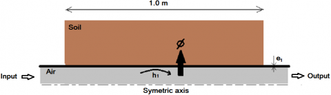
In an EAHE, the process of heat exchanges between the entering air (Tin) and the soil (Tsoil), involves two modes of heat transfers. There is convection inside the pipe and conduction in the pipe material (Figure 1). The heat transmitted per unit of area in each of these transfer modes is respectively given by Eqns. (1) and (2) [20, 21].
Figure 1. Illustration of heat transfer in an Earth-Air Heat Exchanger (EAHE)
$\varphi_{\text {conv }}=\mathrm{h}_{1}\left(\mathrm{~T}_{\mathrm{in}}-\mathrm{T}_{\mathrm{p}}\right)$ (1)
And
$\varphi_{\text {cond }}=-\lambda_{1} \overrightarrow{\text { grad } \mathrm{T}}$ (2)
The terms Tp, h1 and λ1 represent respectively the temperature of the internal face of the duct, the convective heat exchanges coefficient and the thermal conductivity of the duct. Assuming that the air circulates in the pipe of length L, diameter d and thickness e1; the total heat flux transferred by air during its passage through the soil, which is assumed to be an isotropic medium, is given by Eq. (3). Likewise, for a mass air flow $\dot{m}_{a}$ whose temperatures at the inlet and outlet of the duct are respectively Tin and Tout, that same heat flow can be calculated by the relationship given by Eq. (4) [22].
$\emptyset=\pi \mathrm{k}_{1} \mathrm{dL}\left[\mathrm{T}_{\text {in }}-\mathrm{T}_{\text {soil }}\right]$ (3)
with $k_{1}=\frac{1}{r_{1}}$ where $r_{1}=\frac{1}{h_{1}}+\frac{e_{1}}{\lambda_{1}}$.
$\emptyset=\dot{m}_{a} C_{p}\left[T_{\text {out }}-T_{\text {in }}\right]$ (4)
By pooling the above two equations, the expression of the air outlet temperature Tout can be deduced (Eq. (5)). From the data obtained experimentally, the heat transfer coefficient of the exchanger can be determined. The terms ρ and Cp represent the density and specific heat of air, respectively.
$\mathrm{T}_{\text {in }}-\mathrm{T}_{\text {out }}=\frac{4 \mathrm{k}_{1} \mathrm{~L}\left[\mathrm{~T}_{\text {in }}-\mathrm{T}_{\text {soil }}\right]}{\rho d V C_{p}}$ (5)
The coefficient h1 on which k1 depends is a characteristic coefficient of the forced convection of air in the duct. Depending on the speed of air, the diameter of the pipe and its thermal properties, this coefficient can be estimated from the relation given by Eq. (6) established owing to empirical correlations based on dimensionless numbers like the Reynolds (Re), Prandtl (Pr), and Nusselt (Nu) [23, 24]. μ is the dynamic viscosity of air. The thermal properties of the ambient air and the copper duct are given in Table 1.
$\mathrm{h}_{1}=\mathrm{Nu} \frac{\lambda}{\mathrm{d}}$ (6)
$\begin{aligned} \text { If } \operatorname{Re}>5000 \text { then } \mathrm{Nu} &=0.023 \operatorname{Re}^{0.8} \operatorname{Pr}^{0.3} \\ \text { If } \operatorname{Re}<5000 \text { then } \mathrm{Nu} &=1.86(\mathrm{Re} \cdot \operatorname{Pr})^{\frac{1}{3}}\left(\frac{\mathrm{d}}{\mathrm{L}}\right)^{\frac{1}{3}} \\ \text { with: } \operatorname{Re} &=\frac{\rho \cdot \mathrm{v} \cdot \mathrm{d}}{\mu} \\ \text { and } \operatorname{Pr} &=\frac{\mu \cdot C_{\mathrm{p}}}{\lambda} \end{aligned}$
Table 1. Thermal properties of the ambient air and thermal conductivity of the dust material
|
|
Properties |
Values |
|
Air |
$\rho$ |
1.204 kg. $m^{-3}$ |
|
$\lambda$ |
7 $W \cdot m^{-1} \cdot K^{-1}$ |
|
|
$\mu$ |
$1.81 \times 10^{-5}$ Pa.s |
|
|
Cp |
1005 $\mathrm{J} \cdot \mathrm{kg}^{-1} \cdot \mathrm{K}^{-1}$ |
|
|
Pipe |
$\lambda_{1}$ |
386 $\mathrm{W} \cdot \mathrm{m}^{-1} \cdot \mathrm{K}^{-1}$ |
2.2 Experimental approach
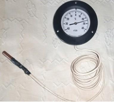
The experimental model (Figure 2) is a heat exchanger implementing the heat transfer between the air circulating in a copper pipe of diameter d = 6.0 mm and length L = 1.0 m, buried in a previously cooled sample of soil. The circulation of air in the pipe is provided by a fan which axially sucks the ambient air and delivers it radially into the circuit which will carry it through the pipe. Three temperature sensors were used, including two type-N thermocouples placed at the inlet (TC1) and outlet (TC2) of the air pipe; and a dial thermometer (TH) of which the probe is buried in the soil sample. Images of these captors are given in Figures 3 and 4 while their characteristics are given in Table 2.
Table 2. Characteristics of the used temperature captors
|
Code |
Sensor name |
Range |
Precision |
|
TC1 |
Thermocouple N |
-200 to 1300℃ |
$\mp$ 0.01℃ |
|
TC2 |
Thermocouple N |
-200 to 1300℃ |
$\mp$ 0.01℃ |
|
TH |
Thermometer |
-40 to 40℃ |
$\mp$ 1℃ |
These sensors are connected to a data acquisition module which is itself connected to a computer. The tests consist of experimenting with the direct exchange of heat between the ambient air passing through the pipe and the cooled soil sample. With a view to investigating the sensitivity of the heat transmission coefficient k, it was a question of varying the soil temperature and the air speed and measuring the inlet and outlet temperatures of air. Figure 5 thus shows the experimental model designed, and on which heat exchange tests were carried out. It was made on the basis of wooden panel of 8 mm in thickness and has external dimensions of 1.032 m x 0.25m x 0.25m. Previously refreshed, the sample of soil used is the sand. The air pipe passing through the sand is copper of 6 mm in diameter and 0.5 mm in thickness.
Figure 2. Outlines of the experimental model implementing the air-soil heat transfer
Figure 3. Inlet and outlet thermocouples connected to the Sensor-PC module
Figure 4. Thermometer used to measure and control the Soil temperature
In view of minimizing the influence of ambient parameters such as temperature and humidity, experiments were carried out during a same period and practically between 11 am and 2 pm so that to have almost a constant humidity during tests. Concerning the effect of ambient temperature in heat transfer, it is important to note that not only the experimental device has been designed with wooden panels, but also an empty space of 6 cm has been left between the inner chamber containing the soil and the outer wall of the exchanger (Figure 6). By controlling the value given by thermometer TH, each test has been made within a negligible variation of the soil temperature.
Figure 5. Front view showing the mockup connected to the computer controlling tests
Figure 6. Interior view showing the empty space between the soil sample and the outer wall
3.1 Response time
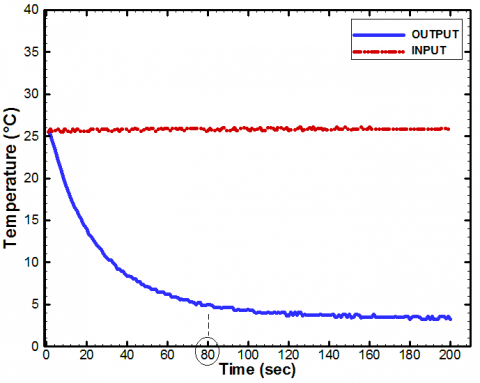
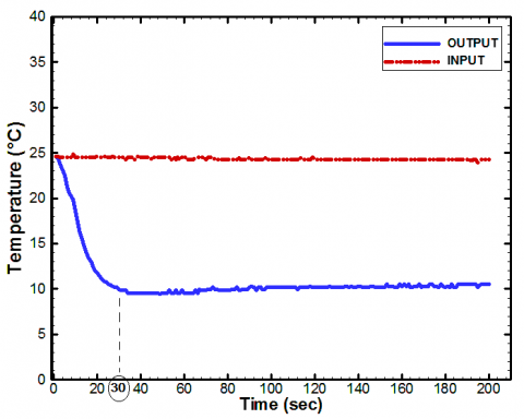
Ambient air was injected into the pipe with respective speeds of 1.2 m/s and 2.9 m/s; with soil samples of average temperatures of 1℃ and 3℃ respectively. The response time, defined as transition point between the unsteady phase and the stationary phase, was deduced for each speed, from the data obtained and which are shown graphically by Figures 7 and 8. On these figures showing the profiles of the inlet and outlet temperatures of the air-soil exchanger as a function of time, it can be noted that the case study with an air injection speed of 2.9 m/s reaches the stationary phase after 30 seconds (Figure 8) while the one with a speed of 1.2 ms-1 reaches it after 80 seconds (Figure 6). This implies that the response time decreases as the air speed in the pipe increases; with an average time step of 29.5 seconds per unit of velocity.
Figure 7. Response time of the case of which the air’s speed is 1.2 m/s
Figure 8. Response time of the case of which the air speed is 2.9 m/s
3.2 Analysis of temperatures
In order to quantifying the energy rate discharged into the soil, once the permanent phase was reached, i.e. the phase where quantities become constant over time, the temperature of the air at the inlet and outlet of the pipe, was measured for 100 seconds. Figure 9 shows the offset curve of outlet temperature of air versus soil temperature. The first obvious remark made is that as the soil temperature decreases, the temperature of the outgoing air also decreases but in a logarithmic manner.
When the air speed is increased to 2.9 m/s, the system behaves in the same way but with a slight increase in the difference between the air temperature at the inlet and the outlet (Figure 10).
Indeed, when the ambient air passes through the soil of average temperature 5℃ with a speed of 1.2 m/s, its average outlet temperature is 11.0℃. When this air passes through the same soil with a speed of 2.9 m/s, its average outlet temperature drops to 9.89℃ (Figure 11); corresponding to a decrease of 1.1℃. This means that the maximization of heat transfer between the air and the soil could be done not only by increasing the exchange surface but also by simply increasing the speed of the air crossing the exchanger. Once average values of experimental data having been calculated, the gap in temperature between the inlet and the outlet air (Tin-Tsoil), as well as the gap in temperature between the inlet air and the soil (Tin-Tsoil), have been determined (Table 3). The use of Eq. (5) allowed determining the corresponding heat transmission coefficients (k1).
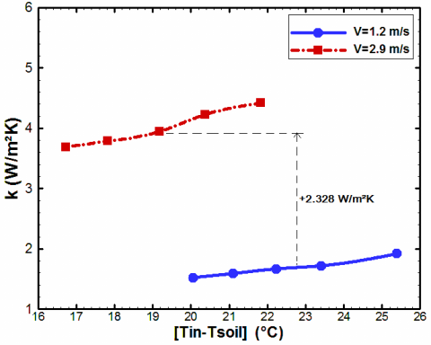
Figure 12 shows, for both speeds, the variation in temperature of the air at the inlet and outlet of the pipe, over the gap temperature between the air and the soil. It is can be seen following both speeds, that the curves are all increasing and have practically the same evolution. This means that (Tin-Tout) grows when (Tin-Tsoil) increases. Although having the same evolution, there is nevertheless a vertical shift in the curve when the air speed goes from 1.2 m/s to 2.9 m/s. That translation of curve reflects an average increase of 2.767℃. This demonstrates once again the sensitivity of heat exchange to the air velocity.
The above analysis highlights the positive effect of velocity on the heat transfer between the fluid and the soil. In reality, velocity influences these heat exchanges through a coefficient called heat transmission coefficient k1. Figure 13 shows the variation of this coefficient according to the soil temperature and the air velocity. It can be noted that this coefficient k1 increases slightly with the soil temperature, but strongly with the air velocity; because for both velocities, curves evolve in the same way according to the soil temperature; but are shifted according to a gap of k1 of 2.328 W/m²K.
Figure 9. Variation of the outlet temperature over the soil temperature: Case of which the air’s speed is 1.2 m/s
Figure 10. Variation of the outlet temperature over the soil temperature: Case of which the air’s speed is 2.9 m/s
Table 3. Summary of the main results obtained over the variation of the air speed and the soil temperature
|
V(m/s) |
TSoil (℃) |
Tout (℃) |
[Tin-Tsoil] (℃) |
[Tin-Tout] (℃) |
K1 (W/m²K) |
|
1.2 |
0.5 |
3.5 $\mp$ 0.3 |
25.4 |
22.4 |
1.92 |
|
2.0 |
7.0 $\mp$ 0.7 |
23.4 |
18.5 |
1.72 |
|
|
3.0 |
8.2 $\mp$ 0.8 |
22.2 |
17.0 |
1.67 |
|
|
4.0 |
9.7 $\mp$ 0.6 |
21.1 |
15.4 |
1.59 |
|
|
5.0 |
11.0 $\mp$ 0.4 |
20.0 |
14.0 |
1.53 |
|
|
2.9 |
6.0 |
9.5 $\mp$ 0.5 |
21.9 |
18.3 |
4.42 |
|
7.0 |
11.0 $\mp$ 0.2 |
20.4 |
16.4 |
4.23 |
|
|
8.0 |
12.8 $\mp$ 0.9 |
19.2 |
14.4 |
3.95 |
|
|
9.0 |
14.0 $\mp$ 0.3 |
17.8 |
12.8 |
3.79 |
|
|
10.0 |
15.0 $\mp$ 0.1 |
16.7 |
11.7 |
3.69 |
Figure 11. Sensitivity of the outlet temperature of air according to the speed inside the duct
Figure 12. Variation of the outlet temperature of air versus the soil temperature
Figure 13. Variation of the heat transmission coefficient versus the soil temperature
3.3 Coupling of effects
The present study focuses on the study of the sensitivity of the outlet temperature of air in an air-soil heat exchanger, following two parameters that are likely varying under actual operating conditions. These two parameters are the soil temperature, which depends on the geographical location of implementation, and the air flow rate in the exchanger, more precisely its speed. Analyses made above have shown in a global way that the air speed in the duct has a positive impact in the heat transfer between the ambient air and the soil. It was thus shown that in laminar flow, the gap temperature between the inlet and outlet air and the heat transmission coefficient increased by 0.653℃ and 1.369 W/m²K per unit of speed, respectively. An equation was used to extract the expression giving the heat transmission coefficient as a function of the flow rate in the exchanger and more precisely its velocity V (Eq. (7)). Since the ratio e1/λ1 is substantially equal to zero, the thermal transmission coefficient k1 is almost equal to the convective coefficient h1.
$k_{1} \approx 1.05 \mu d R e$ (7)
By varying the air flow rate in the duct, the corresponding heat transfer coefficients were calculated using Eqns. (6) and (7) for k1 and k'1 [24], respectively. Substitution of these different values in Eq. (5) allowed the calculation of corresponding temperature gaps; i.e. $\Delta \mathrm{T}$ for the present study and $\Delta \mathrm{T}^{\prime}$ for the literature (Table 4).
Table 4. Comparison of the results obtained from the literature with those obtained using the correlation of the present study
|
V (m.s-1) |
k1 (W/m²k) |
k1’ (W/m²k) |
$\Delta \mathrm{T}$ (℃) |
$\Delta \mathrm{T}^{\prime}$ (℃) |
|
0.294 |
0.457 |
6.318 |
14.562 |
248.461 |
|
0.588 |
0.851 |
7.960 |
13.542 |
156.520 |
|
0.882 |
1.244 |
9.112 |
13.202 |
119.447 |
|
1.176 |
1.637 |
10.029 |
13.032 |
98.601 |
|
1.470 |
2.031 |
10.803 |
12.930 |
84.972 |
|
1.763 |
2.424 |
11.480 |
12.862 |
75.247 |
|
2.057 |
2.817 |
12.085 |
12.813 |
67.898 |
|
2.351 |
3.210 |
12.635 |
12.777 |
62.115 |
|
2.645 |
3.604 |
13.141 |
12.748 |
57.424 |
|
2.939 |
3.997 |
13.611 |
12.726 |
53.529 |
|
3.233 |
4.390 |
14.050 |
12.707 |
50.233 |
|
3.527 |
4.784 |
14.464 |
12.692 |
47.402 |
|
3.821 |
5.177 |
14.855 |
12.678 |
44.939 |
|
4.115 |
5.570 |
15.227 |
12.667 |
42.773 |
|
4.409 |
5.964 |
15.581 |
12.657 |
40.850 |
|
4.702 |
6.357 |
15.920 |
12.649 |
39.130 |
|
4.996 |
6.750 |
16.245 |
12.641 |
37.580 |
|
5.290 |
7.143 |
16.557 |
12.635 |
36.175 |
|
5.584 |
7.537 |
16.858 |
12.629 |
34.894 |
|
5.878 |
7.930 |
17.149 |
12.623 |
33.721 |
|
6.172 |
8.323 |
17.430 |
12.619 |
32.642 |
|
6.466 |
8.717 |
17.702 |
12.614 |
31.645 |
|
6.760 |
9.110 |
17.967 |
12.610 |
30.721 |
|
7.054 |
9.503 |
18.223 |
12.606 |
29.861 |
|
7.348 |
9.897 |
18.473 |
12.603 |
29.060 |
|
7.641 |
10.290 |
18.716 |
12.600 |
28.310 |
|
7.935 |
10.683 |
18.953 |
12.597 |
27.606 |
|
8.229 |
11.076 |
19.184 |
12.594 |
26.945 |
|
8.523 |
11.470 |
19.410 |
12.592 |
26.322 |
|
8.817 |
11.863 |
19.631 |
12.589 |
25.734 |
|
9.111 |
12.256 |
19.846 |
12.587 |
25.177 |
|
9.405 |
12.650 |
20.057 |
12.585 |
24.650 |
|
9.699 |
13.043 |
20.264 |
12.583 |
24.149 |
|
9.993 |
13.436 |
20.467 |
12.581 |
23.674 |
|
10.287 |
13.830 |
20.666 |
12.580 |
23.221 |
|
10.580 |
14.223 |
20.861 |
12.578 |
22.788 |
|
10.874 |
14.616 |
21.052 |
12.577 |
22.376 |
|
11.168 |
15.009 |
21.240 |
12.575 |
21.982 |
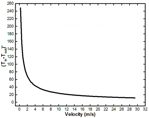
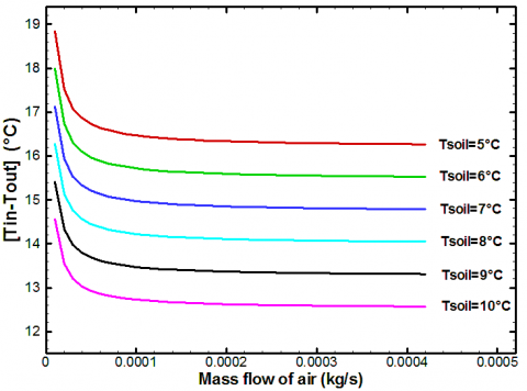
The graphical representation of these temperatures according to the speed shows that the correlation of literature, (Tin-Tout)’ becomes divergent for speeds below 15 m/s (Figure 14); this is no longer compatible with reality because for an inlet temperature Tin = 26℃ and a soil temperature Tsoil = 5℃, the difference (Tin-Tout) must be less than the difference (Tin-Tsoil), i.e. 21℃. Figure 15 presents the variation curve of the output temperature of air when using the heat transmission coefficient k1 deducted from the correlation of the present study. It appears that for speeds below 15 m/s, the model significantly represents reality and admits good performances for speeds below 6 m/s. The representation of the model for different soil temperatures shows a constant increase in efficiency of the exchanger (Figure 16). So as major remark, whatever the soil temperature, the air-soil heat transfer is maximized with low air flow rates.
Figure 14. Variation of (Tin-Tout) versus air velocity: curve obtained with a correlation of h1 deduced from the literature (With Tsoil = 5℃)
Figure 15. Variation of (Tin-Tout) versus air velocity: curve obtained with the correlation of h1 deducted from the present paper (With Tsoil = 5℃)
Figure 16. Variation of the gap of air temperature between the inlet and outlet of the exchanger following the soil temperature
The present study was a description of heat transfer experiments in a bioclimatic air-soil heat exchanger designed for pre-conditioning ambient air before its injection into a building. In order to study the sensitivity of the exchanger in relation to the air velocity and soil temperature, tests were conducted in a device containing previously cooled soil sample through which air had to pass, via a copper pipe, at different speeds. From experimental data obtained, a relation was established expressing the heat transmission coefficient of the exchanger as a function of the air velocity in the pipe. Contrary to correlation existing in the literature, the one established in the present paper fits well to our model of exchanger. However, it is important to reveal that the above results were obtained by using a pipe of length 1.0 m. Next studies will be focused on the varying of the pipe length.
|
Tp |
Temperature of the internal face of duct, ℃ |
|
h1 |
Convective heat coefficient, W.m-2.K-1 |
|
$\lambda_{1}$ |
Thermal conductivity of the duct, W.m-1.K-1 |
|
$\mu$ |
Dynamic viscosity of the air, Pa.s |
|
$\rho$ |
Density of the air, kg.m-3 |
|
Tin |
Temperature of the entering air, ℃ |
|
Tout |
Temperature of out coming air, ℃ |
|
Tsoil |
Temperature of the soil, ℃ |
|
$\varphi_{\text {conv }}$ |
Convection heat per unit of area, W.m-2 |
|
$\varphi_{\text {cond }}$ |
Conduction heat per unit of area, W.m-2 |
|
$\dot{m}_{a}$ |
Mass flow of the air, kg.s-1 |
|
L |
length of the pipe (fixed to 1.0 m) |
|
e1 |
Thickness of the pipe, m |
|
d |
Diameter of the pipe, m |
|
$\varnothing$ |
Heat flux, W |
|
Cp |
Specific heat of the air, J.kg-1.K-1 |
|
V |
Velocity of the air, m.s-1 |
|
Re |
Reynolds number |
|
Pr |
Prandtl number |
|
Nu |
Nusselt number |
[1] International Energy Agency. (2018). Global Energy and CO2 Status Report, IEA.
[2] International Energy Agency. (2012). Activities Report, IEA.
[3] Edenhofer, O., Pichs-Madruga, R., Sokona, Y., Farahani, E., Kadner, S., Seyboth, K., Adler, A., Baum, I., Brunner, S., Eickemeier, P., Kriemann, B., Savolainen, J., Schlömer, S., von Stechow, C., Zwickel, T., Minx, J.C. (2014). Mitigation of climate change: Contribution of working group III to the fifth assessment report of the IPCC. Cambridge University Press.
[4] Goswami, D.Y., Ileslamlou, S. (1990). Performance analysis of a closed-loop climate control system using underground air tunnel. Journal of Solar Energy Engineering, 112: 76-81. https://doi.org/10.1115/1.2929650
[5] Dupui, (2012). The Canadian well: a green and economical solution for preheating or cooling ambient air. Inter-Mecanique du Bâtiment, 27: 12-22.
[6] Musy, A., Soutter, M. (1991). Soil Physics. PPUR Polytechnic Presses.
[7] Mohamed, K. (2016). Contribution to the study of an air-to-ground heat exchanger for air cooling in the hot and semi-arid climate of Marrakech. Doctoral thesis, University of La Rochelle, Maroc.
[8] Thiers, S., Peuportier, B. (2008). Thermal and environmental assessment of a passive building equipped with an earth-to-air heat exchanger in France. Solar Energy, 82(9): 820-831. https://doi.org/10.1016/j.solener.2008.02.014
[9] Vaz, J., Sattler, M.A., Brum, R.D.S., dos Santos, E.D., Isoldi, L.A. (2014). An experimental study on the use of Earth-Air Heat Exchangers (EAHE). Energy and Buildings, 72: 122-131. https://doi.org/10.1016/j.enbuild.2013.12.009
[10] Vaz, J., Sattler, M.A., dos Santos, E.D., Isoldi, L.A. (2011). Experimental and numerical analysis of an earth–air heat exchanger. Energy and Buildings, 43(9): 2476-2482. https://doi.org/10.1016/j.enbuild.2011.06.003
[11] da Silva Brum, R., Vaz, J., Rocha, L.A.O., dos Santos, E.D., Isoldi, L.A. (2013). A new computational modeling to predict the behavior of earth-air heat exchangers. Energy and Buildings, 64: 395-402. https://doi.org/10.1016/j.enbuild.2013.05.032
[12] Santamouris, M., Kolokotsa, D. (2013). Passive cooling dissipation techniques for buildings and other structures: The state of the art. Energy and Buildings, 57: 74-94. https://doi.org/10.1016/j.enbuild.2012.11.002
[13] Soni, S.K., Pandey, M., Bartaria, V.N. (2015). Ground coupled heat exchangers: A review and applications. Renewable and Sustainable Energy Reviews, 47: 83-92. https://doi.org/10.1016/j.rser.2015.03.014
[14] Hollmuller, P., Lachal, B. (2001). Cooling and preheating with buried pipe systems: monitoring, simulation and economic aspects. Energy and Buildings, 33(5): 509-518. https://doi.org/10.1016/S0378-7788(00)00105-5
[15] Hamdi, O., Brima, A., Moummi, N., Nebbar, H. (2018). Experimental study of the performance of an earth to air heat exchanger located in arid zone during the summer period. International Journal of Heat and Technology, 36(4): 1323-1329. https://doi.org/10.18280/ijht.360422
[16] Hollmuller, P. (2002). Use of air-floor heat exchangers for heating and cooling of buildings. Doctoral thesis, University of Geneva, Switzerland.
[17] Olivier, K. (2017). Study of the effectiveness of using a Canadian well to increase the performance of an air-source heat pump. Doctoral thesis, University of Quebec, Montreal.
[18] Nabiha, N. (2009). Analytical study of a water-soil exchanger: 14th international days of thermics. Centre of Research and Technologies of Energy, Tunisia.
[19] Dehina, K., Mokhtari, A. (2012). Numerical simulation of a Co-current air-soil-water exchanger. XXXe Rencontres AUGC-IBPSA, Chambéry, Savoie.
[20] Leleu, R. (1992). Heat Transfers. Editions Techniques de L’Ingénieur.
[21] Incropera, F.P., DeWitt, D.P., Bergman, T.L., Lavine, A.S. (1996). Fundamentals of Heat and Mass Transfer. New York: Wiley.
[22] Saatdjian, S. (2009). The Basics of Fluid Mechanics: Heat and Mass Transfer for the Engineer. Sapientia Editions.
[23] Cheron, B. (1999). Heat Transfers. Edition Ellipses.
[24] Holman, J.P. (1986). Heat Transfer. McGraw-Hill Inc. USA.