Sidi Mohammed Yousfi | Khaled Aliane*
© 2021 IIETA. This article is published by IIETA and is licensed under the CC BY 4.0 license (http://creativecommons.org/licenses/by/4.0/).
OPEN ACCESS
The present work aims to investigate the recirculation and incipient mixing zones in a channel flow supplied with obstacles. The main objective is to develop a new technique to control these recirculation zones by setting a variable roughness. For the purpose of varying that roughness, 4 small bars of heights 0.25H, 0.5H, 0.75H and H were placed downstream of the obstacle; H is the height of the obstacle. For this, a three-dimensional numerical approach was carried out using the ANSYS CFX computer code. In addition, the governing equations were solved using the finite volume method. The K-ω shear-stress transport (SST) turbulence model was utilized to model the turbulent stresses. In the end, we presented the time-averaged simulation results of the contours of the current lines (3D time-averaged streamlines, trace-lines), three components of the velocities: <u> (velocity u contour), <v> (velocity v contour) and <w> (velocity w contour), trace-lines, stream ribbons and mean Q-criterion iso-surface.
turbulent flow, variable roughness, obstacle, finite volume, ANSYS-CFX
Roughness is created artificially by installing a number of obstacles of different shapes and sizes in the flow of a fluid in a channel. For this, a bibliographical analysis was carried out on research works that deal with flows in the presence of obstacles. Over the past few years, a number of experimental and numerical studies have been carried out to investigate and elucidate the complex flows around various, more or less, profiled models [1]. These types of fluid flow are generally found in many industrial applications, such as the cooling of electronic components [2], atmospheric flows around buildings [3], industrial turbines [4], flat plat solar collectors [5, 6], etc. It is worth indicating that several studies have been conducted to understand the vortex structures that develop around obstacles. In this regard, Hussein and Martinuzzi [6] carried out an experimental study of a three-dimensional circulation in a canal containing a cube. The results obtained indicated that the evolution of the turbulence dissipation rate in the recirculation zone was of the same order of magnitude as the asymptotic slip. In another work, Martunizzi and Tropea [7] investigated the flow around prismatic obstacles with different aspect ratios, using techniques that are on crystal violet display, oil film, and laser. The findings suggested that a nominally two-dimensional region existed behind the obstacle and upstream of the recirculation zone. For their part, Hwang and Yang [8] conducted a numerical study on swirl (vortex) structures that develop around a cube placed inside a canal. They found out that the number of vortices increased as the Reynolds number went up. As for Filippini et al. [9], they used the Large Eddy Simulation (LES) model to investigate the instance of a flow around cubes placed into a channel. They found out that when the ratio S/H increased, the average drag coefficient augmented for the second cube while it remained approximately constant for the first one. On the other hand, Lim et al. used the standard Large Eddy Simulation (LES) model to perform a numerical simulation of the flow around an area containing cubes, inside a turbulent boundary layer; the simulation results were then compared with the experimental ones [10, 11]. Using the same approach, Dogan et al. [12], as well as Becker et al. [13], investigated the structure of the flow around three-dimensional obstacles. Moreover, an experimental simulation was conducted using various aspect ratios, in two different types of boundary layers. The experimental results indicated that the flow structure around the obstacle depended on its aspect ratio, angle of attack, Reynolds number, and boundary layer type. On the other hand, Yakhot et al. [14] presented a study of the flow pattern around a surface-mounted cube using the Direct Numerical Simulation (DNS) technique, for a Reynolds number Re = 5160, based on the immersed boundary method. Then, interesting results were obtained using the above mentioned method for the simulation of complex fluid flows. As for Rostane et al. [15], they examined the effect of the curvature of the lower edge of a block placed inside the canal on the aerodynamic phenomena, particularly on the vortex behind the cube. In addition, these same authors investigated the impacts of three curvature radii, i.e. R = 0.2H, R = 0.3H and R = 0.5H, for Re = 105. They found out that the dimensions of the vortex downstream of the obstacle decreased while the curvature radius augmented. Similarly, Aliane and Amraoui [16] examined the influence of roughness created in the insulation of a flat air solar collector in order to increase heat exchange within the collector. Furthermore, Sari-Hassoun and Aliane [17] performed a numerical analysis of the flow around a block placed inside a rectangular channel, using two models of obstacles: a rectangular cube and a similar one with rounded upstream edge; they used the k-ε turbulence model. Salim et al. [18] developed an approach to treat turbulent flows over a surface-mounted cube using the wall stress (y+ wall) as a guide to select the appropriate grid pattern and the corresponding turbulence models. For this, they used the Fluent calculation code. The study was divided into two parts: the first one used a low Reynolds number and the second one a high Reynolds number. On the other hand, Heguehoug et al. [19] conducted a study on a turbulent, stationary, three-dimensional and incompressible flow, without any heat transfer around an isolated 3D profile and through a series of 60 blades that were part of a fixed wheel, similar to that of a turbomachine. Moreover, Merahi et al. [20] carried out a study that contributed to understanding the three-dimensional stationary and incompressible flow through a cascade of blades using a numerical simulation based on the k-ε model; they found out that the pressure losses due to the change in the angle of incidence are the main causes of the decline in the performance of turbomachines. Similarly, Amraoui and Aliane [21, 22] investigated the fluid flow and heat transfer inside a solar flat plate collector using Computational Fluid Dynamics (CFD) by introducing suitable baffles inside the solar air collectors in order to decrease the pressure losses and increase the temperature. As regards Dogan et al. [12], they examined the characteristics of a flow around a surface-mounted cube for Re = 3700 using the Computational Fluid Dynamics (CFD), while considering three different types of turbulence models; the results obtained were then compared with the experimental ones. Haidary et al. [23] investigated the pool boiling heat transfer of water over cylindrical heating tubes for different orientations and surface roughness of the tubes. Two orientations of a smooth heating tube, horizontal and vertical, were used in the boiling chamber. For their part, Kanfoudi et al. [24] employed the large eddy simulation (LES) to perform a numerical analysis of the turbulent flow structure induced by the cavitation shedding. In addition, Djeddi et al. [25] conducted a simulation of a viscous fluid flow over an unconventional diamond-shaped obstacle inside a confined channel, for low to moderate Reynolds numbers. For this, the diamond-shaped obstacle was geometrically modified to represent different blockage coefficients, depending on the height of the channel and for different aspect ratios, based on the obstacle's length-to-height ratios. The simulations were performed for two steady and unsteady flow groups. Moreover, Liakos et al. [26] performed a Direct Numerical Simulation (DNS) of a steady-state laminar flow over a cube for Reynolds numbers ranging from 1 to 2000, depending on the height of the cube. The same authors examined the topologies as well as the development of the fluid around the obstacle. Avdhoot and Alangar [27] investigated the transient boiling characteristics on a rough copper sample that possesses a surface roughness value (Ra) within the interval from 0.106 μm to 4.03 μm. Moreover, the effect of roughness and time constant of the exponential heat supply on the transient critical heat flux (CHF), maximum heat transfer coefficient (HTC) and onset of nucleate boiling (ONB) was extensively investigated as well. In addition, Sumner et al. assessed the effects of the aspect ratio and incidence angle on the flow structure above the free ends of a surface-mounted finite-height circular cylinder and a finite-height square prism [28, 29]. Regarding Shinde et al. [30], they performed a large eddy simulation of a flow over a wall-mounted cube-shaped obstacle placed in a spatially evolving boundary layer for the purpose of understanding how variations in the cube height can modify the flow dynamics in the case where the cube is inside the boundary layer. Likewise, Ennouri et al. [31] carried out the modelling and simulation of the flow inside a centrifugal pump, under cavitation and non-cavitation conditions, using the SST-SAS turbulence model. Similarly, Zakaria et al. [32] implemented an experimental study on a flat plate air solar collector. They found out that mini concentrators (curved obstacles) contributed enormously to the performance improvement of a flat plate solar air collector. Similarly, Rostane et al. [33] studied the effect of a hole in the center of a cube by considering four three-dimensional obstacle configurations for the analysis of the flow around this cube embedded in a surface for a Reynolds number Re = 40 000. The SST k-omega turbulence model was used in the ANSYS CFX programming code. The findings revealed the presence of a second vortex behind the obstacles with a dimensionless ratio of the hole diameter D over the obstacle height H (D/H = 0.2). It should be noted that the turbulence kinetic energy was quite large in the case of an obstacle without a hole. However, in the presence of a hole, the turbulence kinetic energy started decreasing as the diameter of the hole increased. The drag coefficient increased only when the ratio D/H was equal to 0.32. On the other hand, Benahmed and Aliane [34] investigated the effect of the two upper inclined edges of a rectangular cube on the flow structure. Afterwards, a three-dimensional study was conducted using the ANSYS CFX calculation code, and the turbulence models were applied to analyse the characteristics of the flow around the inclined obstacle.
The present work aims to investigate the influence of the variable roughness that is placed downstream of an obstacle on the occurrence of mixing and circulation zones in the region that is closest to the obstacle.
The averaged mass and momentum conservation equations are expressed as:
$\frac{\partial \rho }{\partial t}+\frac{\partial \left( \rho {{U}_{i}} \right)}{\partial {{x}_{i}}}=0$ (1)
$\frac{\partial {{U}_{i}}}{\partial t}+{{U}_{j}}\frac{\partial {{U}_{i}}}{\partial {{x}_{j}}}=-\frac{1}{\rho }\frac{\partial P}{\partial {{x}_{i}}}+v\frac{{{\partial }^{2}}{{U}_{i}}}{\partial {{x}_{j}}\partial {{x}_{j}}}$ (2)
In addition, the Reynolds equation is expressed as:
$\rho \frac{\partial {{{\bar{U}}}_{i}}}{\partial t}+\rho {{\bar{U}}_{j}}\frac{\partial {{{\bar{U}}}_{i}}}{\partial {{x}_{j}}}=-\frac{\partial \bar{P}}{\partial {{x}_{i}}}+\frac{\partial }{\partial {{x}_{j}}}\left( \mu \frac{\partial \overline{{{U}_{i}}}}{\partial {{x}_{j}}}-\rho \overline{{{u}^{\prime }}iu_{j}^{\prime }} \right)$ (3)
The SST (Shear Stress Transport) k- ω turbulence model of Menter [35] was used in this study; it was derived from the Standard k-ω model [36]. This model combines the robustness and accuracy of the k-ω model in the near-wall region of the channel with the k-ε model [37] and all free-flow related types, away from the wall. The SST k-w model is mainly recommended for applications where the fluids undergo sudden stress changes and flow around curved surfaces, or in the case of boundary layer separation. Therefore, the SST k-omega turbulence model may be considered as ideal for our simulation.
The turbulent viscosity was modified so as to take into account the transport of turbulent shear flow.
The formulation of the two-equation turbulence model is:
$\rho \frac{\partial k}{\partial t}+\rho {{\bar{U}}_{j}}\frac{\partial k}{\partial {{x}_{j}}}={{\tilde{P}}_{k}}-\rho {{C}_{\mu }}\omega k+\frac{\partial }{\partial {{x}_{j}}}\left[ \left( \mu +{{\mu }_{t}}/{{\sigma }_{k}} \right)\frac{\partial k}{\partial {{x}_{j}}} \right]$ (4)
The specific dissipation rate is given as:
$\begin{align} & \rho \frac{\partial \omega }{\partial t}+\rho {{{\bar{U}}}_{j}}\frac{\partial \omega }{\partial {{x}_{i}}}=2\alpha \rho {{S}_{ij}}{{S}_{ij}}-\beta \rho {{\omega }^{2}}+ \\& \frac{\partial }{\partial {{x}_{j}}}\left[ \left( {{\mu }_{t}}+{{\sigma }_{\omega }}{{\mu }_{t}} \right)\frac{\partial \omega }{\partial {{x}_{j}}} \right]+2\left( 1-{{F}_{1}} \right)\rho {{\sigma }_{\omega 2}}\frac{1}{\omega }\frac{\partial k}{\partial {{x}_{j}}}\cdot \frac{\partial \omega }{\partial {{x}_{j}}} \\\end{align}$ (5)
As for the blending function F1, it is defined using the following equation:
${{F}_{1}}=\tanh \left\{ {{\left\{ \min \left[ \max \left( \frac{\sqrt{k}}{{{C}_{\mu }}\omega L},\frac{500v}{{{L}^{2}}\omega } \right),\frac{4\rho {{\sigma }_{\omega 2}}k}{C{{D}_{k\omega }}{{L}^{2}}} \right] \right\}}^{4}} \right\}$ (6)
In the near-wall region, F1=1; however it goes to zero in the outer region $C D_{k \omega}$ that is given as:
$\mathop{CD}_{k\omega }=\max \left( 2\rho \mathop{\sigma }_{\omega 2}\frac{1}{\omega }\frac{\partial k}{\mathop{\partial x}_{j}}.\frac{\partial \omega }{\mathop{\partial x}_{j}},\mathop{10}^{-10} \right)$ (7)
Moreover, the eddy viscosity is expressed as:
${{v}_{t}}=\frac{{{\alpha }_{1}}k}{\max \left( {{\alpha }_{1}}\omega ,\sqrt{2}{{S}_{ij}}{{F}_{2}} \right)}$ (8)
The second blending function F2 is defined by the following equation:
${{F}_{2}}=\tanh \left[ {{\left[ \max \left( \frac{2\sqrt{k}}{{{C}_{\mu }}\omega L},\frac{500v}{L{{\omega }^{2}}} \right) \right]}^{2}} \right]$ (9)
To prevent the accumulation of turbulence in the stagnation regions, it was decided to limit the production of turbulence:
${{\tilde{P}}_{k}}=\min \left( {{P}_{k}},10.{{C}_{\mu }}\rho k\omega \right)$ (10)
${{P}_{k}}={{\mu }_{t}}\frac{\partial {{U}_{i}}}{\partial {{x}_{j}}}\left( \frac{\partial {{U}_{i}}}{\partial {{x}_{j}}}+\frac{\partial {{U}_{j}}}{\partial {{x}_{i}}} \right)$ (11)
The model constants are calculated using the blending function below:
$F1:\phi ={{F}_{1}}{{\phi }_{1}}+\left( 1-{{F}_{1}} \right){{\phi }_{2}}$ (12)
The values of the model constants are: $C_{\mu}=0.09, \alpha_{1}=5 / 9$, $\alpha_{2}=0.44, \beta_{2}=0.0828, \sigma_{\mathrm{k}_{1}}=0.85, \sigma_{\mathrm{k}_{2}}=1.0, \sigma_{\omega_{1}}=0.5$ and $\sigma_{\omega_{2}}=0.856$.
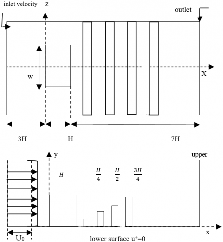
The geometric model used in this work is represented by a cubic-shaped obstacle of height (H), as shown in Figure 1. A variable roughness was added downstream of the obstacle in order to disturb the boundary layer at that position and enhance the dynamic and thermal exchanges. The obstacle and the variable roughness were placed in a horizontal channel of length (11H), height (2H) and width L = 7H. The variable roughness consisted of four small bars. Note that the length of each bar is equal to the channel width (7H). These bars all have the same width (0.5H). Their heights are successively equal to (0.25H), (0.5H), (0.75H) and (H). The distance between two successive bars is equal to (0.5H), as depicted in Figure 2.
Figure 1. Three-dimensional view of the computational domain of the geometry
Figure 2. Geometry of computational domain and boundary conditions
As the flow is turbulent, the SST k-ω turbulence model was chosen to analyse the problem. In this case, all walls were taken as adiabatic, with no-slip conditions. According to the previously selected model, the equations should be solved using the following parameters: The incoming flow velocity U0 corresponds to the Reynolds number 8.104 (Re = U0.h/) and the channel height (h). The height of the obstacle was H = 25 mm, and the channel height was h = 2H. The velocity was zero (u = 0 m/s) near the lower and upper walls of the channel and above the obstacle. Moreover, the roughness was varied. A constant pressure was imposed at the outlet of the channel such that Pout = 0.
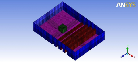
For the purpose of achieving highly accurate results, it was necessary to generate a well refined mesh. For this, it was deemed interesting to opt for a structured hexahedral mesh. The meshing of the domain was performed using ANSYS CFX. The general practice consists of using a fine mesh size in regions where the domain geometries undergo small changes. Figure 3 shows the mesh grid used.
Figure 3. The mesh grid configuration
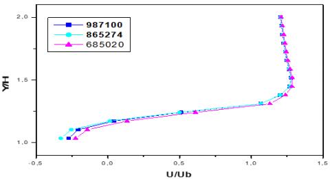
The grid independence was investigated using a series of simulation tests within the calculation domain corresponding to the velocity under consideration.
Table 1. Different meshing sizes
|
|
L/H |
h/H |
Grid |
|
Configuration 1 |
7 |
2 |
685020 |
|
Configuration 2 |
7 |
2 |
865274 |
|
Configuration 3 |
7 |
2 |
987100 |
Figure 4. Testing the grid sensitivity
For this, several mesh sizes were tested (Figure 4) in order to attain results that are independent of the number of meshes. Consequently, three meshes with hexahedral elements and sizes 685020, 865274 and 987100 were used. The values reported in Table 1 correspond to the situation where x /H= 0.5. The findings of this study showed that there are comparatively small differences between the three grids. Eventually, the mesh including 865274 elements was chosen as the best solution with regard to precision and calculation time.
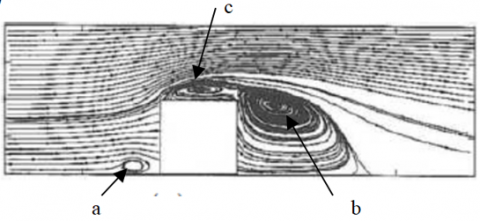
The flow above the wall-mounted cube (without roughness) engenders complex phenomena such as horseshoe vortices and recirculation zones on the top and back of the cube, as illustrated in Figure 5. It is worth noting that the presence of the obstacle causes the fluid flow to separate near the upstream face of the obstacle. The flow forms a recirculation zone near this face, which causes the turbulence intensity to augment. In addition to the separation of the fluid flow in the three zones (X1, X2 and X3), the fluid velocity also increases in this region because the cross-sectional area of the fluid passage gets narrower at that point. Note that the length of the recirculation zone on the upper face of the cube is represented by X2 in Figure 5. The flow separation takes place on the upstream and downstream edges of the cube. A large separation region develops downstream (X2) and upstream (X1) of the cube. The effect of the separation (X1) on the flow adds up to that of the horseshoe vortex. The length of this region is represented by X1.
Figure 5. Flow pattern around an inclined cube attached to the wall with three vortex lengths
In this study, the experimental flow model carried out experimentally by Martinuzzi and Tropea (1993) was considered for the purpose of validating the characteristics of the flow over the surface-mounted cube (without roughness) placed in a channel of height h = 2H; the height of the cube was H = 25 mm. The structure of the flow around the obstacle was validated by the work of Hussein and Martinuzzi (1995) for a Reynolds number Re = 8.0×10⁴ (Figure 6a). This part of the fluid, which is blocked between the lower wall of the channel and the front face of the obstacle, leads to zero speed in that region, which explains the appearance of this small recirculation zone. Upstream of the obstacle, part of the fluid remained blocked, forming a small recirculation zone (point (a) in the case of Hussein and Martinuzzi (1995) and point (a') in our case Figure 6b). Downstream of the obstacle, a large vortex appeared, as is clearly shown in the two figures (point (b) in the case of Hussein and Martunizzi and point (b') in our case). This was due to the strong depression of the flow in that region, which engendered a return current (vortex). The separation occurred above the obstacle; this was caused by the stopping point upstream of the obstacle (point of separation) (point (c) in the case of Hussein and Martunizzi and point (c') in our case). At that point, the flow accelerates due to the presence of the obstacle which leads to the constriction of the flow passage section. A simple comparison between the two simulations allowed concluding that the results obtained are satisfactory and encouraging.
(a) Hussein and Martinuzzi (1995)
(b) SST k-ω
Figure 6. Streamlines velocity on the symmetry plane for Re= 8.104
In this study, the influence of surface roughness on the flow structure was subsequently examined. For this, a three-dimensional study was carried out using the ANSYS CFX calculation code. The size of the computational domain is 11H × 7H × 2H. The inlet of the computational field, which is located at a distance of 3H upstream of the cube; note that the fully developed velocity profiles were used, with a Reynolds number (Reh=Ubh/ν) equal to 8.0×10⁴. At the outlet of the canal, a constant pressure pout = pref was maintained. In addition, no-slip conditions were imposed at the solid walls (upper surface, lower surface, and cube). In this case, the side boundaries were considered as slip surfaces, while considering the symmetry conditions. The hexahedral structured meshes were employed for solving the fluid dynamics equations (Figure 3).
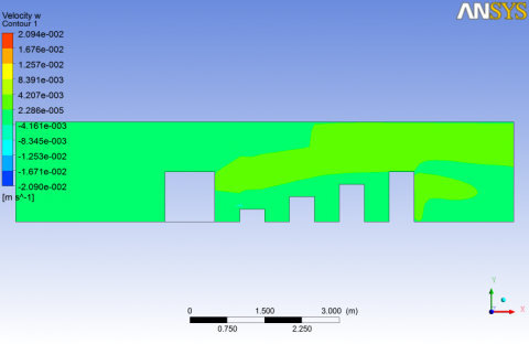
It is worth indicating that the SST K-ω turbulence model was used to study the characteristics of the flow around the cube with a rough surface for a Reynolds number Re = 8.104. The normalized time-averaged results of the longitudinal velocity <u>, and the transversal velocity components <v> and <w> on the symmetry plane (z = 0) around the obstacle are all presented in Figure 7.
The stream-wise velocity is clearly depicted in Figure 7. This figure allows observing that the velocity is low around the cube and along the roughness bars. This velocity increased and reached its maximum value downstream of the fourth and last bar in the region close to the upper wall. It is minimal at the exit of the channel in the lower zone of the channel. The cross-stream velocity component <v > for Re = 8.104 is explicitly shown in Figure 7. The maximum values of the cross-stream velocity were reached upstream of the cube where part of the fluid remained blocked due to the presence of the obstacle, which caused the velocity to increase. Likewise, it was observed that the velocity increased also above the first three roughness bars. The minimum values were more predominant downstream of the last bar and at the exit of the canal. This same Figure 7 also indicates that the velocity component <w> was very negligible, i.e. nearly equal to zero inside the major part of the canal, except downstream of the obstacle where the velocity was quite low.
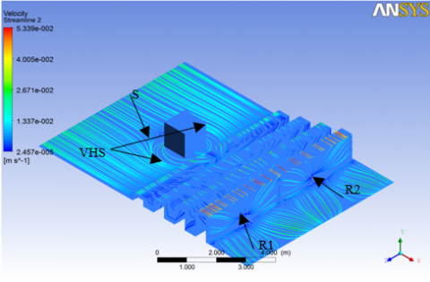
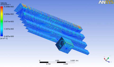
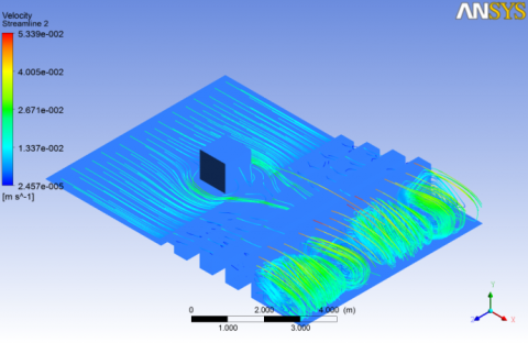
Figure 8 was used to conduct an accurate analysis of the flow. Moreover, the flow separation and reattachment phenomena on the top of, at the lateral sides of, and behind the obstacle, as well as the time-averaged streamlines near the channel floor for the Reynolds number Re = 8.104 are clearly illustrated as well.
Figure 7. Components of velocity vectors <u>, <v> and <w> on the symmetry plane (z=0) at Re = 8.104
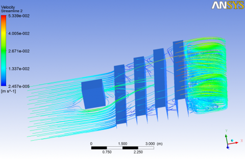
Figure 8. Time-averaged streamlines at the floor of the channel at the Reynolds number of Re=8.104
It is worth indicating that the blocking effect due to the obstacle created an unfavorable pressure gradient that was responsible for the separation of the flow, and then moved away from the cube, forming a horseshoe vortex that appeared upstream and bypassed the obstacle; it is represented by the point (VHS). On the other hand, two reattachment points (R1, R2) were observed on the last roughness bar, as well as a separation point (S) upstream of the cube.
7.1 Trace-lines
Figure 9 shows trace-lines on the surface of the cube as well as on the surfaces of the four bars representing the roughness on the bottom wall of the channel. These trace-lines suggested that there was a regular flow on the upper faces of both the cube and the bars. A flow separation was observed at the middle of the front face of the obstacle, thus forming a node and a recirculation zone on the lateral faces of this cube. Similarly, a flow circulation zone was observed on the front faces of the four roughness bars.
7.2 Stream-ribbons
Figure 10 shows the stream-ribbons as well as a along with a large vortex and a recirculation zone downstream of the last roughness bar. A flow separation was also observed upstream of the cube due to the presence of the obstacle. It can therefore be concluded that the separation region around a three-dimensional body cannot be closed.
7.3 Mean Q-criterion iso-surface
The Q-criterion is a new way to visualize turbulent flows.
This criterion is a scalar invariant that is defined by the expression: $\mathrm{Q}=-\frac{1}{2} \mathrm{Ui}, \mathrm{j} \mathrm{Uj}, \mathrm{i}=-\left(\left\|\mathrm{S}^{2}\right\|-\left\|\Omega^{2}\right\|\right)[38]$. In addition, the Q-criterion can be dimensioned using the expression: $\bar{Q}=$ $\mathrm{Q} /(\mathrm{Ub} / \mathrm{H}) 2 .$
Figure 9. Trace-lines on the surface of the cube and the four roughness bars
(a) Front view
(b) Lateral view
(c) Rear view
Figure 10. Stream-ribbons
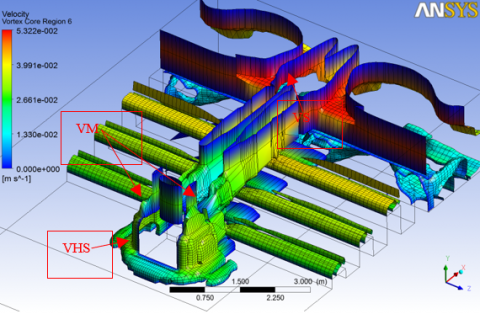
Figure 11 clearly depicts the three-dimensional structure of the flow, in particular the presence of a horseshoe vortex upstream of the cube, noted VHS, in addition to marginal vortices noted VM and wake vortex noted VS. One may also observe that the fluid was reflected immediately after the last roughness bar.
Figure 11. Iso-outline of mean Q-criterion
This work was an attempt to analyze a three dimensional turbulent flow around an obstacle with a variable roughness that was located downstream of that obstacle. For this, an interactive three-dimensional approach was applied using the ANSYS CFX Calculation Code. In addition, the governing equations were solved using the finite-volume method. Moreover, the shear-stress transport (SST) K- ω turbulence model was utilized to study the characteristics of the flow around the cube with rough surfaces, for the Reynolds number Re = 8.104. This work sought to study the recirculation zones as well as the incipient mixing in a flow, in the presence of a cubic obstacle. The main purpose was to develop a new technique for controlling these recirculation zones by adding a variable roughness, represented by four bars of different heights, i.e. 0.25H, 0.5H, 0.75H and H, placed downstream of the obstacle on the bottom wall of the channel. The velocity was found quite low around the cube and the roughness bars. Moreover, it turned out that this velocity increased and reached its maximum value downstream of the fourth and last bar in the region close to the upper wall. Its minimal value was found at the exit of the channel, and in the lower zone of the channel. The maximum values of the cross-stream velocity were achieved upstream of the cube where part of the fluid remained blocked due to the presence of the obstacle. The blocking effect of the obstacle created an unfavorable pressure gradient which separated the flow and moved away from the cube; this allowed the formation of a horseshoe vortex upstream of the obstacle and then bypassed the obstacle; it is represented by the point (VHS). On the other hand, two reattachment points (R1, R2) were detected on the last roughness bar and a separation point (S) was observed upstream of the cube. Furthermore, a flow separation was noticed in the middle of the front face of the obstacle, which contributed to the formation of a node and a recirculation zone on the lateral faces of the cube. In addition, a circulation zone was observed on the front faces of the four roughness bars. Flow separation was noticed upstream of the cube due to the presence of the obstacle. Therefore, it can be concluded that the separation region around a three-dimensional body cannot be closed.
[1] Aliane, K. (2011). Passive control of the turbulent flow over a surface-mounted rectangular block obstacle and a rounded rectangular obstacle. International Review of Mechanical Engineering, 5(2): 305-314.
[2] Nemdili, S., Nemdili, F., Azzi, A. (2015). Improving cooling effectiveness by use of chamfers on the top of electronic components. Microelectronics Reliability, 55: 1067-1076. http://dx.doi.org/10.1016/j.microrel.2015.04.006
[3] Diaz-Daniel, C., Laizet, S., Vassilicos, J. C. (2017). Direct numerical simulations of a wall-attached cube immersed in laminar and turbulent boundary layers. International Journal of Heat and Fluid Flow, 68: 269-280. https://doi.org/10.1016/j.ijheatfluidflow.2017.09.015.
[4] Aliane K., Sebbane O., Hadjoui A. (2003). Dynamic study of turbomachine blade cooling models. Proceedings of the 11th International Day of Thermomics, Algiers (Algeria), pp. 315-320.
[5] Amraoui, M.A., Aliane, K. (2018). Three-dimensional analysis of air flow in a flat plate solar collector. Periodica Polytechnica Mechanical Engineering, 62(2): 126-135. https://doi.org/10.3311/PPme.11255
[6] Hussein, H.J.A., Martinuzzi, R.J. (1996). Energy balance for turbulent flow around a surface mounted cube placed in a channel. Physics of Fluids, 8(3): 764-780. https://doi.org/10.1063/1.868860
[7] Martinuzzi, R., Tropea, C. (1993). The flow around a surface-mounted prismatic obstacle placed in a fully developed channel flow. J. Fluids Eng., 115: 85-92. https://doi.org/10.1115/1.2910118
[8] Hwang, J.Y., Yang, K.S. (2004). Numerical study of vortical structures around a wall-mounted cubic obstacle in channel flow. Physics of Fluids, 16(7): 2382-2394. https://doi.org/10.1063/1.1736675
[9] Filippini, G., Franck, G., Nigro, N., Storti, M., D’Elía, J. (2005). Large eddy simulations of the flow around a square cylinder. Mecanica Computacional, 1279-1298.
[10] Lim, H.C., Thomas, T.G., Castro, I.P. (2009). Flow around a cube in a turbulent boundary layer: LES and experiment. Journal of Wind Engineering and Industrial Aerodynamics, 97(2): 96-109. https://doi.org/10.1016/j.jweia.2009.01.001
[11] Krajnovic, S., Davidson, L. (2002). Large-eddy simulation of the flow around a bluff body. AIAA Journal, 40(5): 927-936. https://doi.org/10.2514/2.1729
[12] Dogan, S., Yagmur, S., Goktepeli, I., Ozgoren, M. (2017). Assessment of turbulence models for flow around a surface-mounted cube. International Journal of Mechanical Engineering and Robotics Research, 6(3): 237-241. https://doi.org/10.18178/ijmerr.6.3.237-241
[13] Becker, S., Lienhart, H., Durst, F. (2002). Flow around three-dimensional obstacles in boundary layers. Journal of Wind Engineering and Industrial Aerodynamics, 90(4-5): 265-279. https://doi.org/10.1016/S0167-6105(01)00209-4
[14] Yakhot, A., Liu, H., Nikitin, N. (2006). Turbulent flow around a wall-mounted cube: A direct numerical simulation. International Journal of Heat and Fluid Flow, 27(6): 994-1009. https://doi.org/10.1016/j.ijheatfluidflow.2006.02.026
[15] Rostane, B., Aliane, K., Abboudi, S. (2015). Three dimensional simulation for turbulent flow around prismatic obstacle with rounded downstream edge Using the k-ω SST model. International Review of Mechanical Engineering, 9(3): 266-277. https://doi.org/10.15866/ireme.v9i3.5719
[16] Aliane, K., Amraoui, M. (2013). Etude numérique d’un capteur solaire plan à air ayant une rugosité rectangulaire. Journal of Renewable Energies, 16(1): 129-141.
[17] Sari-Hassoun, Z., Aliane, K. (2016). Simulation numérique de l’écoulement turbulent autour d’obstacles a arête amont courbé. International Journal of Scientific Research & Engineering Technology, 4: 196-201.
[18] Salim, M., Ariff, M., Cheah, S.C. (2009). Wall y+ Approach for Dealing with Turbulent Flows over a Surface Mounted Cube: Part 2 - High Reynolds Number. Seventh International Conference on CFD in the Minerals and Process Industries CSIRO, Melbourne, Australia.
[19] Heguehoug, K., Nemouchi, Z., Gaci, F. (2010). Contribution à l’étude de l’écoulement Tridimensionnel turbulent autour d’un profil et à travers une série d’aubes fixes, TERMOTEHNICA.
[20] Merahi, I., Abidat, M., Azzi, A., Hireche, O. (2002). Numerical assessment of incidence losses in an annular blade cascade, Séminaire international de Génie Mécanique, Sigma’02 ENSET, Oran.
[21] Amraoui, A., Aliane, K. (2014). Dynamic and thermal study of the three-dimensional flow in a flat plate solar collector with transversal baffles. International Review of Mechanical Engineering (IREME), 8(6): 1030-1036. https://doi.org/10.15866/ireme.v8i6.1623
[22] Amraoui, A., Aliane, K. (2014). Numerical analysis of a three dimensional fluid flow in a flat plate solar collector. International Journal of Renewable and Sustainable Energy, 3(3): 68-75. https://doi.org/10.11648/j.ijrse.20140303.14
[23] Haidary, F.M., Hasan, M.R., Adib, M., Labib, S.H., Hossain, M.J., Ghosh, A.K., Goswami, A. (2021). Enhancement of pool boiling heat transfer over plain and rough cylindrical tubes. International Journal of Heat and Technology, 39(2): 329-339. https://doi.org/10.18280/ijht.390201
[24] Kanfoudi, H., Bellakhall, G., Ennouri, M., Taher, A.B. H., Zgolli, R. (2017). Numerical analysis of the turbulent flow structure induced by the cavitation shedding using LES. Journal of Applied Fluid Mechanics, 10(3): 933-946. https://doi.org/10.18869/acadpub.jafm.73.238.27384
[25] Djeddi, S.R., Masoudi, A., Ghadimi, P. (2013). Numerical simulation of flow around diamond-shaped obstacles at low to moderate Reynolds numbers. American Journal of Applied Mathematics and Statistics, 1(1): 11-20. https://doi.org/10.12691/ajams-1-1-3
[26] Liakos, A., Malamataris, N.A. (2014). Direct numerical simulation of steady state, three dimensional, laminar flow around a wall mounted cube. Physics of Fluids, 26(5): 053603. https://doi.org/10.1063/1.4876176
[27] Avdhoot, W., Alangar, S. (2019). Experimental Investigation on transient pool boiling heat transfer from rough surface and heat transfer correlations. International Journal of Heat and Technology, 37(2): 545-554. https://doi.org/10.18280/ijht.390201
[28] Sumner, D., Rostamy, N., Bergstrom, D., Bugg, J. (2015). Influence of aspect ratio on the flow above the free end of a surface-mounted finite cylinder. International Journal of Heat and Fluid Flow, 56: 290-304. https://doi.org/10.1016/j.ijheatfluidflow.2015.08.005
[29] Sumner, D., Rostamy, N., Bergstrom, D., Bugg, J.D. (2017). Influence of aspect ratio on the mean flow field of a surface-mounted finite-height square prism. International Journal of Heat and Fluid Flow, 65: 1-20. https://doi.org/10.1016/j.ijheatfluidflow.2017.02.004
[30] Shinde, S., Johnsen, E., Maki, K.J. (2017). Understanding the effect of cube size on the near wake characteristics in a turbulent boundary layer. In 47th AIAA Fluid Dynamics Conference, Denver, Colorado. https://doi.org/10.2514/6.2017-3640
[31] Ennouri, M., Kanfoudi, H., Bel Hadj Taher, A., Zgolli, R. (2019). Numerical flow simulation and cavitation prediction in a centrifugal pump using an SST-SAS turbulence model. Journal of Applied Fluid Mechanics, 12(1): 25-39. https://doi.org/10.29252/jafm.75.253.28771
[32] Zakaria, S., Khaled, A., Mustapha, H. (2017). Experimental study of a flat plate solar collector equipped with concentrators. International Journal of Renewable Energy Research (IJRER), 7(3): 1028-1031.
[33] Rostane, B., Khaled, A., Abboudi, S. (2019). Influence of insertion of holes in the middle of obstacles on the flow around a surface-mounted cube. Journal of Computational & Applied Research in Mechanical Engineering (JCARME), 9(1): 77-87. https://doi.org/10.22061/JCARME.2019.3984.1472
[34] Benahmed, L., Aliane, K. (2019). Simulation and analysis of a turbulent flow around a three-dimensional obstacle. Acta Mechanica et Automatica, 13(3): 173-180. http://dx.doi.org/10.2478/ama-2019-0023
[35] Menter, F. (1994). Two-equation eddy-viscosity. turbulence models for engineering application. AIAA Journal, 32: 1598-1605. https://doi.org/10.2514/3.12149
[36] Bitsuamlak, G., Stathopoulos, T., Bedard, C. (2006). Effects of upstream two-dimensional hills on design wind loads a computational approach. Wind and Structures, 9(1): 37-58. https://doi.org/10.12989/was.2006.9.1.037
[37] Hadjoui, A., Sebbane, O., Aliane, K., Azzi, A. (2003). Study of the appearance of swirling zones in a flow confronted with obstacles located at the entrance of a canal, Proceedings of the 9th Congress of the French Society of Process Engineering, Saint-Nazaire, France, pp. 224-229.
[38] Hunt, J.C.R., Wray, A.A., Moin, P. (1988). Eddies, stream and convergence zones in turbulent flows. Center of Turbulence Research, 193-208.