Xiling Gao* | Libin Shang | Rujie Xia | Xiaodong Zhang | Wei Yao
© 2021 IIETA. This article is published by IIETA and is licensed under the CC BY 4.0 license (http://creativecommons.org/licenses/by/4.0/).
OPEN ACCESS
Taking the bed in the bedroom as an air-conditioning system (ACS), this paper attempts to disclose the influence of air supply height (ASH) on sleep comfort. Specifically, a computational fluid dynamics (CFD) model was established to simulate the air temperature distribution, air speed, and carbon dioxide content (CDC) indoor at five ASHs of the ACS. The simulation results were compared with lab data. On this basis, the aeration efficiency (AE), temperature regulation risk (TRR), and energy-use factor (EUF) of the ACS were analyzed under different working conditions, and the overall efficacy of the ACS was assessed comprehensively by the technique for order of preference by similarity to ideal solution (TOPSIS).
air supply height (ASH), sleep comfort, computational fluid dynamics (CFD), aeration efficiency (AE), technique for order of preference by similarity to ideal solution (TOPSIS)
In tropical or subtropical regions, hot and humid summer usually lasts more than 7 months a year. Air conditioners must be turned on around the clock to create a good indoor environment for sleeping. Unsurprisingly, air-conditioning systems (ACSs) in tropical or subtropical regions consume more and more electricity, taking up a growing portion in the power consumed by buildings [1]. The building designers in these regions must pursue power-efficient air-conditioning, without sacrificing indoor thermal comfort.
Task air-conditioning (TAC) [2] is an ACS composed of multiple working positions. In the working area, the temperature, humidity, and pollutant content can be adjusted by controlling various parameters. TAC is capable of maintaining a comfortable microenvironment through effective use of energy. As a result, the system has been widely used in office buildings and residential buildings.
Many scholars discovered that TAC helps to create a sleep environment, because most beds cover a very limited space [3]. Some of themoptimized sleep environment with bed-centric TAC system, and realized power-efficient temperature regulation [4]. Someadapted TAC system to real bedrooms, and measured its aeration efficiency (AE), temperature regulation risk (TRR), and energy-use factor (EUF).
The above analysis shows the importance to further explore the TAC system, aiming to ensure indoor thermal comfort without consuming too much electricity [5]. With the aid of computational fluid dynamics (CFD) software [6], the authors analyzed the VE, TRR, and EUF at various air supply heights (ASHs) of bedroom ACS, and comprehensively evaluated the overall efficacy, AE, temperature regulation effect [7], and power efficiency of bedroom TAC.
2.1 Geometric model
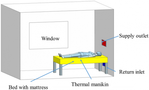
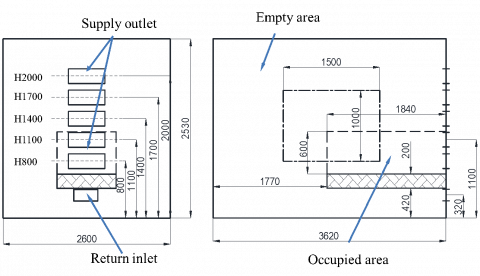
Figure 1 shows the geometric model of the target bedroom [8]. The dimensions of the bedroom are displayed in Figure 2. Several ASHs of the bedroom ACS were considered: 800mm, 1,100mm, 1,400mm, 1,700mm, and 2,000mm.
Figure 1. Geometric model of the target bedroom (ASH=1, 100mm)
Figure 2. Dimensions of the bedroom
2.2 Meshing
Before CFD simulation, it is critical to mesh the computational domain into suitable grids. Since the target bedroom has a simple structure, this paper decides to mesh the empty and occupied areas separately into a few structured grids [9] (Figure 3).
(a) Grids of the bedroom
(b) Grids of manikin surface
Figure 3. Grids of the geometric model
2.3 Mathematical model
The continuity and energy equations of three-dimensional (3D) steady state Reynolds-averaged Navier-Stokes (RANS) approach [10] were introduced to compute the air flow and thermal convection in the computational domain. The SST turbulence model [11] was coupled with the second-order upwind scheme of k-omega and k-epsilon models into a simple algorithm to solve the governing equations. The algorithm performs well in the prediction of air speed and thermal distribution indoor.
The equation of the conservation of mass was adopted to forecast the indoor distribution of carbon dioxide content (CDC) [12]:
$\nabla\left(\rho \vec{u} Y_{i}\right)-\nabla \vec{J}_{i}=S_{i}$ (1)
$\vec{J}_{i}=-\left(\rho D_{i, m}+\frac{\mu_{t}}{S_{c t}}\right) \nabla Y_{i}-D_{T, i} \frac{\nabla T}{T}$ (2)
Drawing on empirical evidence, the air supply temperature was set to 21-27℃, air supply volume to 20-110L/s, fresh air volume to 6.5-13L/s. Each simulation deals with nine cases. In total, 45 cases were compared to reveal the AE, TRR, and EUF under changing air supply volume, air supply temperature, and fresh air volume, such as to comprehensively evaluate the performance of bedroom TAC system.
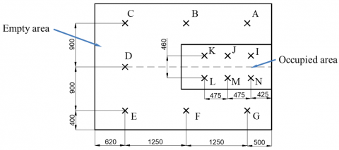
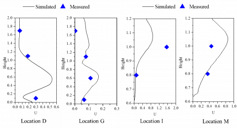
To verify the CFD approach, an ACS with ASH=1,100mm was modeled for simulation. Figure 4 shows the measuring points of air temperature, air speed, and mean CDC of the manikin and unoccupied area at D, G, I, and M.
Figure 4. Measuring points
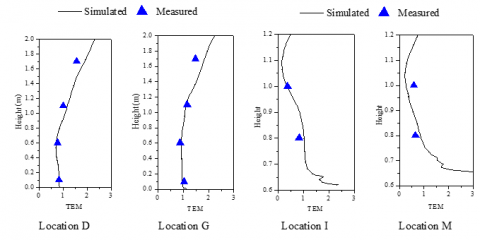
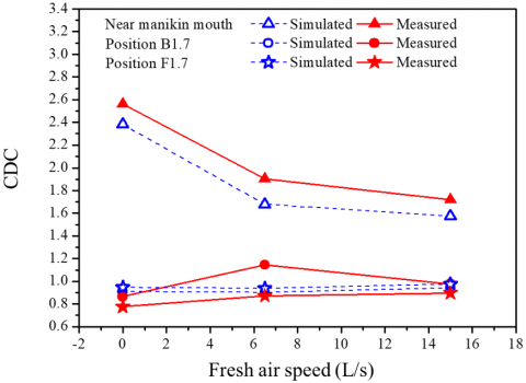
Figures 5-7 compare simulated parameters with actual parameters. It can be learned that the simulated parameters agree well with the actual ones. Overall, the simulated air temperature and air speed were consistent with the actual data in the empty area. As for CDC, the CDC near the mouth of the manikin was simulated under multiple speeds of the fresh air. The simulated CDC values were basically the same as the actual values. Hence, the CFD simulation is accurate enough to forecast the air temperature, air speed, and CDC in the computational domain.
Figure 5. Simulated air temperature vs. actual air temperature
Figure 6. Simulated air speed vs. actual air speed
Figure 7. Simulated CDC vs. actual CDC
This paper evaluates the operating performance of the ACS in the sleep environment with AE, TRR, and EUF [13]. Among them, AE can be calculated by [14]:
$A E=\frac{C_{r}-C_{S}}{C_{O Z}-C_{S}}$ (3)
Once the ACS enters operation, a cold wind will sweep across the sleep environment. Then, the TRR of the ACS [15] can be calculated by:
$T R R=(34-t)(v-0.05)^{0.62}\left(0.37 v T_{u}+3.14\right)$ (4)
Note that any $v \leq 0.05 \mathrm{~m} / \mathrm{s}$ should be treated as $v=0.05$ $\mathrm{m} / \mathrm{s}$, and any $T R R>100 \%$ should be taken as $T R R=100 \%$.
Suppose the mean air temperature remains the same. The higher the temperature, the greater the power efficiency. Hence, the EUF of the ACS can be calculated by [16]:
$E U F=\frac{\left(t_{u z}-t_{s}\right)}{\left(t_{o z}-t_{s}\right)}$ (5)
The EUF>1 indicates that the occupied area is on average hotter than the empty area. The higher the EUF, the better the power efficiency.
Table 1 shows the CFD simulation results on AE, TRR and EUF. On this basis, the ACS performance was assessed in two steps: assessing against each of the three indices; evaluating the overall utility of the CAS by TOPSIS.
5.1 Single-index assessment
(a) Different fresh air speeds
(b) Different air supply speeds
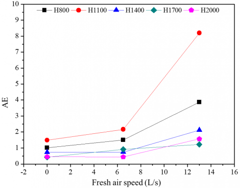
Figure 8. Simulated AE vs. actual AE
Figure 8 compares the simulated AE with the actual AE. As fresh air speed increased, the best AE was achieved under ASH=1,100mm, followed closely by ASH=800mm. With the growth of air supply volume, ASH=800mm realized the best AE, followed by ASH=1,100mm.
(a) Different air supply speeds
(b) Different air supply temperatures
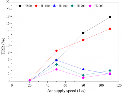
Figure 9. Simulated mean TRR vs. actual TRR
Table 1. CFD simulation results
|
Working condition |
ts (℃) |
Qs (L/s) |
Qf (L/s) |
Case |
||||
|
H800 |
H1100 |
H1400 |
H1700 |
H2000 |
||||
|
1 |
21 |
50 |
6.5 |
1.1 |
2.1 |
3.1 |
4.1 |
5.1 |
|
2 |
23 |
20 |
6.5 |
1.2 |
2.2 |
3.2 |
4.2 |
5.2 |
|
3 |
23 |
50 |
6.5 |
1.3 |
2.3 |
3.3 |
4.3 |
5.3 |
|
4 |
23 |
80 |
6.5 |
1.4 |
2.4 |
3.4 |
4.4 |
5.4 |
|
5 |
23 |
110 |
6.5 |
1.5 |
2.5 |
3.5 |
4.5 |
5.5 |
|
6 |
23 |
50 |
0 |
1.6 |
2.6 |
3.6 |
4.6 |
5.6 |
|
7 |
23 |
50 |
13 |
1.7 |
2.7 |
3.7 |
4.7 |
5.7 |
|
8 |
25 |
50 |
6.5 |
1.8 |
2.8 |
3.8 |
4.8 |
5.8 |
|
9 |
27 |
50 |
6.5 |
1.9 |
2.9 |
3.9 |
4.9 |
5.9 |
Figure 9 compares the simulated TRR with the actual TRR. ASH=800mm and ASH=1,100mm had higher mean TRR than the other three ASHs. Under these two ASHs, the TRR rose sharply with the growing air supply speed. By contrast, the TRR remained low under any of the other three ASHs. Besides, the change of mean TRR comes from the air supply temperature variation with ASHs. The rising air supply temperature helps to suppress TRR.
(a) Different air supply speeds
(b) Different air supply temperatures
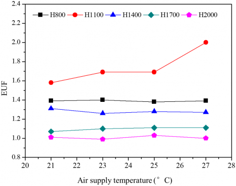
Figure 10. Simulated EUF vs. actual EUF
Figure 10 compares the simulated EUF with the actual EUF. Under different air supply volumes and temperatures, ASH=800mm and ASH=1,100mm achieved better power efficiency than the other ASHs, especially with the rise of air supply volume. The reason is that, at a low ASH, a high air supply volume brings lots of cold air to cool down the occupied area. When the ASH was 2,000mm, the area needed to be cooled with a huge amount of cold air.
To sum up, AE is affected by the volume of air supply and that of fresh air; TRR and EUF depend on the temperature and volume of air supply. As the air supply speed accelerated from 20 to 110L/s, the EUF increased by 1.19 under ASH=8,00mm, and dropped by 0.18 under ASH=2,000mm. When ASH was 800mm, a higher volume of air supply brought a higher TRR in the occupied area, indicating that TRR is negatively correlated with air supply volume. By contrast, the growth of air supply volume led to a higher EUF, i.e., better power efficiency.
5.2 Overall utility assessment
The overall utility of the ACS cannot be fully assessed with a single index. Thus, the comprehensive evaluation tool TOPSIS was introduced to assess the overall utility of the ACS with all the three indices through the following steps:
Step 1. Normalize the original values of the three indices in each case;
Step 2. Multiply the normalized values with the corresponding index weights;
Step 3. Obtain a positive ideal solution to each case on the basis of the weighted values;
Step 4. Sort the cases by the positive ideal solutions.
The ranking of a case is positively correlated with the similarity score, and the overall utility of the case [17].
Index weighting is a key link of TOPSIS. For the ACS, the weight reflects the importance of each index in the assessment of overall utility of the system. Here, each index is weighed both objectively and subjectively (Table 2).
Table 2. Index weights
|
Weighing method |
Importance ranking |
Weights |
||||
|
AE |
TRR |
EUF |
||||
|
Objective |
Entropy |
- - |
0.55 |
0.4 |
0.05 |
|
|
Subjective |
Analytic hierarchy process (AHP) |
AV1 |
AE>TRR>EUF |
0.54 |
0.3 |
0.16 |
|
AV2 |
AE>EUF>TRR |
0.54 |
0.16 |
0.3 |
||
|
AD1 |
TRR>AE>EUF |
0.3 |
0.54 |
0.16 |
||
|
AD2 |
TRR>EUF>AE |
0.16 |
0.54 |
0.3 |
||
|
AE1 |
EUF>AE>TRR |
0.3 |
0.16 |
0.54 |
||
|
AE2 |
EUF>TRR>AE |
0.16 |
0.3 |
0.54 |
||
Inspired by entropy theory [18], each index was weighed by the reciprocal of its divergence. As shown in Table 2, AE and TRR had much greater weights than EUF, that is, the former two change much more violently than EUF. Hence, the variation of EUF was ignored.
The subjective approach is AHP [19], which transforms natural thoughts into a clear process, using a relational scale. Each level of the scale represents a degree of importance. Here, each index is rated by multiple respondents. Therefore, six importance levels were designed for each of the three indices. Table 2 lists the weights of the indices under each level.
The importance of the three indices under all six levels was synthetized into a matrix of three rows and three columns (Table 3). The largest eigenvalue of the matrix corresponds to the eigenvector (0.847, 0.466, 0.257). Based on the eigenvector, the weights of AE, TRR, and EUF were derived as 0.54, 0.30, and 0.16, respectively.
Table 3. Matrix at importance level AV1
|
Index |
AE |
TRR |
EUF |
|
AE |
1(AE/AE) |
1(AE/TRR) |
3(AE/EUF) |
|
TRR |
1/2(TRR/AE) |
1(TRR/TRR) |
2(TRR/EUF) |
|
EUF |
1/3(EUF/AE) |
1/2(EUF/TRR) |
1(EUF/EUF) |
5.2.1 Overall utility in each case
Table 4 sorts the cases by the similarity score obtained through TOPSIS. Under most conditions, Case 2.7 was the best case, thanks to its good aeration performance and excellent power efficiency. But the temperature regulation of the case for AD2 was merely acceptable.
The EUF had a very small weight, according to the entropy theory. The small weight weakens the superiority in power efficiency at ASH=800mm and 1,100mm. The ranking was relatively low in the two cases, owing to the relatively high risk.
AHP results suggest that the overall utility of the cases varied with priorities. For AV2, ASH=800mm and 1,100mm ranked high by their ideal results of AE and EUF. As shown in Figure 10, Cases 1.4, 1.5, 2.7, and 2.9 achieved relatively good aeration performance and high ranking, with large volumes of fresh air and air supply.
Moreover, the high-ranking cases were not greatly influenced by TRR or EUF, namely, Cases 1.5 and 2.7. The overall ranking for AV1 and AV2 was very similar. For AD1 and AD2, the overall ranking was high for ASHs with low air supply volume or high ASHs with low TRR, such as Cases 1.2, 2.2., 3.2, 4.2, and 5.2.
Furthermore, the changes in the relative importance of EUF may greatly affect the overall ranking. Taking Case 2.7 for example, the overall ranking for AD1 was 1 and that for AD2 was 31. This is because the superiority of AE could not make up for the defect of TRR, when AE has a low weight.
For AE1 and AE2, the overall ranking of the cases hinges on the second index. When TRR was less important than AE, high rankings were achieved by the cases with ASH=800mm or ASH=1,100mm, or with a high fresh air speed. When TRR was more important than AE, high rankings were achieved by the cases with a small air supply volume, and a large ASH, such as Cases 1.2, 2.2, 3.2, 4.2 and 5.2.
5.2.2 Overall utility under each ASH
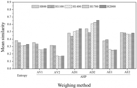
To assess the overall utility of the ACS under each ASH, the similarity of all the cases was averaged under each ASH (Figure 11).
As shown in Figure 11, following the entropy method, the mean similarities were close to each other under the five ASHs, and the greatest mean similarity was observed under ASH=800mm; following the AHP, the mean similarity varied with importance levels.
When AE was the most important index (AV1 and AV2), ASH=800mm and 1,100mm achieved higher mean similarities than the other ASHs, owing to their excellent ventilation effects. In particular, TRR was the least important index for AV2. In this case, the advantage of ASH=800mm and 1,100mm in mean similarity was exceedingly prominent over the other ASHs. This is because the two ASHs suppresses the negative effect of TRR.
When TRR was the most important index (AD1 and AD2), ASH=1,400mm, 1,700mm, and 2,000mm achieved relatively high mean similarities, for their TRRs were rather small.
Table 4. Similarity ranking of cases
|
ASH |
Case number |
Entropy |
AHP |
|||||
|
AV1 |
AV2 |
AD1 |
AD2 |
AE1 |
AE2 |
|||
|
H800 |
1.1 |
36 |
36 |
21 |
36 |
37 |
23 |
38 |
|
1.2 |
7 |
9 |
19 |
4 |
3 |
20 |
8 |
|
|
1.3 |
27 |
23 |
14 |
30 |
30 |
14 |
22 |
|
|
1.4 |
4 |
4 |
3 |
42 |
43 |
3 |
24 |
|
|
1.5 |
2 |
2 |
2 |
43 |
44 |
2 |
31 |
|
|
1.6 |
35 |
37 |
32 |
32 |
32 |
25 |
28 |
|
|
1.7 |
3 |
3 |
4 |
3 |
22 |
4 |
3 |
|
|
1.8 |
18 |
16 |
13 |
20 |
21 |
13 |
11 |
|
|
1.9 |
13 |
11 |
12 |
12 |
11 |
12 |
4 |
|
|
H1100 |
2.1 |
43 |
41 |
17 |
41 |
41 |
15 |
42 |
|
2.2 |
12 |
15 |
22 |
7 |
5 |
22 |
9 |
|
|
2.3 |
25 |
14 |
6 |
38 |
39 |
8 |
25 |
|
|
2.4 |
42 |
29 |
9 |
44 |
42 |
6 |
37 |
|
|
2.5 |
45 |
38 |
10 |
45 |
45 |
9 |
45 |
|
|
2.6 |
41 |
39 |
15 |
40 |
40 |
11 |
34 |
|
|
2.7 |
1 |
1 |
1 |
1 |
31 |
1 |
1 |
|
|
2.8 |
21 |
12 |
8 |
23 |
35 |
7 |
13 |
|
|
2.9 |
5 |
5 |
5 |
24 |
27 |
5 |
2 |
|
|
H1400 |
3.1 |
44 |
45 |
44 |
39 |
38 |
42 |
43 |
|
3.2 |
10 |
13 |
20 |
6 |
4 |
21 |
7 |
|
|
3.3 |
39 |
42 |
41 |
35 |
34 |
37 |
39 |
|
|
3.4 |
33 |
35 |
40 |
25 |
20 |
43 |
35 |
|
|
3.5 |
19 |
22 |
29 |
14 |
10 |
28 |
16 |
|
|
3.6 |
38 |
43 |
42 |
34 |
33 |
38 |
40 |
|
|
3.7 |
11 |
6 |
7 |
23 |
28 |
10 |
20 |
|
|
3.8 |
32 |
31 |
31 |
27 |
24 |
27 |
23 |
|
|
3.9 |
20 |
20 |
23 |
15 |
13 |
18 |
10 |
|
|
H1700 |
4.1 |
40 |
44 |
43 |
37 |
36 |
45 |
44 |
|
4.2 |
8 |
10 |
18 |
5 |
2 |
19 |
6 |
|
|
4.3 |
34 |
34 |
33 |
29 |
25 |
34 |
32 |
|
|
4.4 |
17 |
21 |
30 |
13 |
9 |
31 |
17 |
|
|
4.5 |
26 |
28 |
37 |
19 |
17 |
39 |
30 |
|
|
4.6 |
37 |
40 |
45 |
31 |
29 |
44 |
41 |
|
|
4.7 |
28 |
25 |
24 |
28 |
26 |
32 |
36 |
|
|
4.8 |
22 |
24 |
28 |
18 |
16 |
30 |
19 |
|
|
4.9 |
16 |
19 |
25 |
11 |
8 |
24 |
12 |
|
For AE1, ASH=800mm and 1,100mm achieved relatively high mean similarities, by virtue of their good AE and power efficiency. For AE2, it is hard to tell which ASH led to the optimal performance, because the five ASHs had very close mean similarities. For instance, a TRR was generated under ASH=800mm and 1,100mm, despite their good AE and power efficiency. In the other three ASHs, the low TRRs were realized at the cost of poor AE and power efficiency. Overall, when AE is the second important index, the ACS performance is roughly the same under all ASHs.
Figure 11. Mean similarity of all cases under each ASH
(1) When AE is the most important index, the overall utility of the ACS can be optimized under the following parameter combination: ASH=1,100mm; air supply temperature, 23℃; air supply volume, 50L/s; fresh area volume, 13L/s.
(2) When the index weights are determined by entropy method (objective approach), the overall utility of the ACS improves with the decrease of ASH; when the weights are determined by AHP (subjective approach), the overall utility of the ACS varies with the importance levels of the three indices: If TRR is the most important index, the system performance will improve with ASH; if AE or EUF is the most important index, the system performance will improve with the reduction of ASH.
(3) The authors introduced TOPSIS to assess the ACS performance at each of the five ASHs under various working conditions, and discovered that the performance ranking depends on index weights. In particular, when AHP is adopted, the index weights are greatly affected by the preference of evaluators. The evaluated performance of the ACS will change with the different index weights assigned by different evaluators.
This paper is supported by Youth Fund Project, Jiangsu Provincial Collaborative Innovation Center (No: SJXTQ1504); Science and Technology Project, Jiangsu Provincial Department of Housing and Urban-rural Development (No: 2019ZD001149).
[1] Borowski, M., Łuczak, R., Halibart, J., Zwolińska, K., Karch, M. (2021). Airflow fluctuation from linear diffusers in an office building: The thermal comfort analysis. Energies, 14(16): 4808. https://doi.org/10.3390/EN14164808
[2] Mao, N., Pan, D., Chan, M., Deng, S. (2015). Parameter optimization for operation of a bed-based task/ambient air conditioning (TAC) system to achieve a thermally neutral environment with minimum energy use. Indoor and Built Environment, 26(1): 132-144. https://doi.org/10.1177/1420326X15608678
[3] Or, O.O.Y. (2020). Implementation of online questionnaires in the General Household Survey in Hong Kong. Statistical Journal of the IAOS, 36(4): 987-995. https://doi.org/10.3233/SJI-200746
[4] Emad, A., Khalil, E.E., Elharriry, G., Aboudeif, T.M. (2020). Thermal comfort and air flow patterns in cruise ships. In AIAA Propulsion and Energy 2020 Forum, p. 3940. https://doi.org/10.2514/6.2020-3940
[5] Zaki, S.A., Rosli, M.F., Rijal, H.B., Sadzli, F.N.H., Hagishima, A., Yakub, F. (2021). Effectiveness of a cool bed linen for thermal comfort and sleep quality in air-conditioned bedroom under hot-humid climate. Sustainability, 13(16): 9099. https://doi.org/10.3390/SU13169099
[6] Patel, A., Dhakar, P.S. (2018). CFD analysis of air conditioning in room using ansys fluent. Journal of Emerging Technologies and Innovative Research, 5(11): 436-441. https://doi.org/10.13140/RG.2.2.13462.50249
[7] Kajurek, J., Rusowicz, A., Grzebielec, A., Bujalski, W., Futyma, K., Rudowicz, Z. (2019). Selection of refrigerants for a modified organic Rankine cycle. Energy, 168: 1-8. https://doi.org/10.1016/J.ENERGY.2018.11.024
[8] Fang, G., Deng, S., Liu, X. (2021). A numerical study on evaluating sleeping thermal comfort using a Chinese-Kang based space heating system. Energy and Buildings, 111174. https://doi.org/10.1016/J.ENBUILD.2021.111174
[9] Nehasil, O., Dobiášová, L., Mazanec, V., Široký, J. (2021). Versatile AHU fault detection–Design, field validation and practical application. Energy and Buildings, 237: 110781. https://doi.org/10.1016/J.ENBUILD.2021.110781
[10] Guenther, J., Sawodny, O. (2018). Versatile ventilation and air conditioning operation: Gaussian process regression for temperature field prediction. In 2018 Annual American Control Conference (ACC), pp. 5262-5267. https://doi.org/10.23919/ACC.2018.8431040
[11] Erb, A., Hosder, S. (2021). Analysis and comparison of turbulence model coefficient uncertainty for canonical flow problems. Computers & Fluids, 105027. https://doi.org/10.1016/J.COMPFLUID.2021.105027
[12] Fan, X., Salama, A., Sun, S. (2020). A locally and globally phase-wise mass conservative numerical algorithm for the two-phase immiscible flow problems in porous media. Computers and Geotechnics, 119: 103370. https://doi.org/10.1016/J.COMPGEO.2019.103370
[13] Liu, W., Lian, Z., Yao, Y. (2008). Optimization on indoor air diffusion of floor-standing type room air-conditioners. Energy and Buildings, 40(2): 59-70. https://doi.org/10.1016/J.ENBUILD.2007.01.010
[14] Alguliyev, R.M.O., Aliguliyev, R.M., Mahmudova, R.S. (2015). Multicriteria personnel selection by the modified fuzzy VIKOR method. The Scientific World Journal. https://doi.org/10.1155/2015/612767
[15] Persily, A. (2015). Challenges in developing ventilation and indoor air quality standards: The story of ASHRAE Standard 62. Building and Environment, 91: 61-69. https://doi.org/10.1016/J.BUILDENV.2015.02.026
[16] Singh, S. (2017). Performance evaluation of a novel solar air heater with arched absorber plate. Renewable Energy, 114: 879-886. https://doi.org/10.1016/J.RENENE.2017.07.109
[17] Shekhovtsov, A., Salabun, W. (2020). A comparative case study of the VIKOR and TOPSIS rankings similarity. Procedia Computer Science, 176: 3730-3740. https://doi.org/10.1016/J.PROCS.2020.09.014
[18] Aguarón, J., Escobar, M.T., Moreno-Jiménez, J.M. (2021). Reducing inconsistency measured by the geometric consistency index in the analytic hierarchy process. European Journal of Operational Research, 288(2): 576-583. https://doi.org/10.1016/J.EJOR.2020.06.014
[19] Šoja, S.J., Anokić, A., Jelić, D.B., Maletić, R. (2016). Ranking EU countries according to their level of success in achieving the objectives of the sustainable development strategy. Sustainability, 8(4): 306. https://doi.org/10.3390/SU8040306