Qiuyu Bo | Wuqun Cheng* | Tong Sun
© 2021 IIETA. This article is published by IIETA and is licensed under the CC BY 4.0 license (http://creativecommons.org/licenses/by/4.0/).
OPEN ACCESS
Nowadays, people are paying increasing attention to the rational exploitation of geothermal resources. To develop and utilize geothermal resources in a scientific way, it is important to understand the change patterns of key geohydrological parameters such as seepage velocity and temperature. As part of the effort, this paper analyzes and studies the influencing mechanism of geothermal fluids on the dynamic changes of groundwater flow and heat transfer temperature. First, a differential equation of heat conduction of geothermal fluids and a groundwater flow-geothermal fluids thermal coupling model were constructed to study the seepage state and the heat transfer of groundwater flow in the energy extraction process. Then, an analytical model for the influence of groundwater seepage on heat transfixion was established, directly showing the relevant mechanism. The experimental results proved the effectiveness of the constructed model.
geothermal, groundwater flow, flow rate, temperature field
Energy consumption and environmental protection are two major issues which countries around the world have attached great importance to and been concerned about [1-5]. The increasing use of mineral energy has caused serious environmental problems such as the greenhouse effect and acid rain, so it is imperative and also of great social significance to develop renewable energy resources such as geothermal energy, water energy, air energy and solar energy [6-11]. Geothermal resources have such advantages as high thermal energy utilization efficiency, short development time and immediate availability, so how to rationally exploit them has received increasing attention [12-15]. To develop and utilize geothermal resources in a scientific way, it is important to understand some geohydrological parameters, especially seepage velocity and temperature.
Based on the results of regional hydrogeological survey, Ilko et al. [16] elaborated the applicable conditions and the application case of the 3D groundwater flow numerical simulation method, and gave the particle tracking algorithm flow for groundwater flowline applicable for groundwater flow pattern analysis. Fujii et al. [17] constructed an attribute parameter system of source and sink items and aquifers in the region and a zoning map. With the aid of the software Visual MODFLOW, it solved the constructed 3D groundwater flow numerical simulation model and performed optimization inversion of the parameters. Observation holes in the area were used to monitor the groundwater level dynamics and flow field. Based on the Morris method, Phuoc et al. [18] numerically simulated the permeability coefficient, water supply and permeability of groundwater flow, and plotted the parameter sensitivity distribution contour map for the identification of regional groundwater sensitive and insensitive areas. Shulyupin et al. [19] took a regional groundwater heat pump system project as an example and simulated and analyzed the coupled groundwater flow-heat transfer process under specific heat source conditions. Based on the basic principle of groundwater heat transfer, Qiao et al. [20] analyzed the coupling effect of aquifer flow transfixion and heat transfixion and constructed a numerical simulation model for groundwater flow field and temperature field, and also gave the basis for flow transfixion of groundwater flow when the hydraulic slope is neglected. Ovando-Chacon et al. [21] performed a case analysis of a regional groundwater heat pump system project, and analyzed and evaluated the simulation results of the coupled groundwater flow-heat transfer process under different influencing factors and the sustainable operation schemes.
Scholars at home and abroad have conducted a lot of research on the geothermal energy technology in recent years, but there are still a number of problems demanding prompt solutions, such as the thermal pollution in recharges with large temperature differences, the incomplete recharge of groundwater flow and the interferences between heat outlets [22-25]. The changes in the temperature of geothermal fluids greatly affect the physical, chemical and biological evolution of groundwater flow and even the water quality. Therefore, this paper analyzes and studies the influencing mechanism of geothermal fluids on the dynamic changes of groundwater flow and heat transfer temperature. The paper is organized as follows: in Section 2, a differential equation of heat conduction of geothermal fluids is established; in Section 3, a groundwater flow-geothermal fluids thermal coupling model was constructed to study both the seepage state and the heat transfer of groundwater flow in the energy extraction process; in Section 4, an analytical model is established to directly show the influence of groundwater seepage on heat transfixion. The effectiveness of the constructed model is proved by the experimental results.
During the exploitation of geothermal resources, the geothermal pumping and recharging process will cause changes in the attributes of the groundwater flow in aquifers and its temperature, and the changes in groundwater flow temperature will greatly affect the geothermal energy utilization efficiency. Dynamic changes in water seepage or excessive temperature changes can also lead to changes in the complex geothermal environment. Therefore, it is necessary to analyze the dynamic characteristics of groundwater flow and the changes in heat transfer temperature.
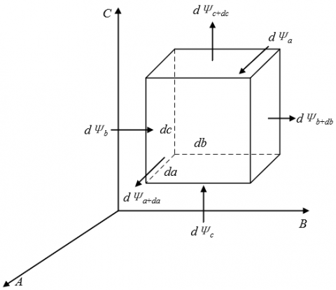
Figure 1. Heat absorption and release of a microelement from geothermal fluids
Suppose the geothermal fluids and groundwater flow under study are isotropic continuous media with internal heat sources. Let the thermal conductivity be denoted as μ, the specific heat capacity as BR, the density as γ, the heat released by a unit volume of geothermal fluids in a unit time period dt, which characterizes the intensity of the internal heat source, as eu. Let a micro-element with three sides parallel to the a, b and c axes split out from the geothermal fluids that generate heat during the pumping and recharge process be du=dadbdc. Figure 1 shows a schematic diagram of the heat absorption and release of the microelement from the geothermal fluids. Based on the law of conservation of energy, the sum of the heat generated by the heat source and the net heat absorbed and released by the micro-element within the dt period should be equal to the increase in the thermodynamic energy of the micro-element.
By summation of the heat absorbed and released by the micro-element along the axes a, b and c, the net heat absorbed and released by the micro-element is obtained. The heat absorbed by the micro-element along the a-axis within the dt time is obtained by Formula (1):
$d{{\Psi }_{a}}={{e}_{a}}dbdcdt$ (1)
The heat released by the micro-element from the surface a+da is obtained by Formula (2):
$d{{\Psi }_{a+da}}={{e}_{a+da}}dbdcdt$ (2)
where, ea+da can be obtained by Formula (3):
${{e}_{a+da}}={{e}_{a}}+\frac{\partial {{e}_{a}}}{\partial a}da$ (3)
The net heat absorbed and released by the micro-element along the a-axis within the dt time is:
$d{{\Psi }_{a}}-d{{\Psi }_{a+da}}=-\frac{\partial {{e}_{a}}}{\partial a}dadbdcdt$ (4)
Similarly, the net heat absorbed and released by the micro-element along the b-axis within the dt time is:
$d{{\Psi }_{b}}-d{{\Psi }_{b+db}}=-\frac{\partial {{e}_{b}}}{\partial b}dadbdcdt$ (5)
The net heat absorbed and released by the micro-element along the c-axis is:
$d{{\Psi }_{c}}-d{{\Psi }_{c+dc}}=-\frac{\partial {{e}_{c}}}{\partial c}dadbdcdt$ (6)
Combine Formulas (4), (5) and (6), and the net heat NH absorbed and released by the micro-element is:
$NH=-\left( \frac{\partial {{e}_{a}}}{\partial a}+\frac{\partial {{e}_{b}}}{\partial b}+\frac{\partial {{e}_{c}}}{\partial c} \right)dadbdcdt$ (7)
As ea, eb and ec are the projections of the vector e on the a, b and c axes, the above formula can be converted to:
$NH=\left[ \frac{\partial }{\partial a}\left( \mu \frac{\partial h}{\partial a} \right)+\frac{\partial }{\partial b}\left( \mu \frac{\partial h}{\partial b} \right)+\frac{\partial }{\partial c}\left( \mu \frac{\partial h}{\partial c} \right) \right]dadbdcdt$ (8)
The heat generated by the internal heat source in the micro-element within the dt time is:
$IH={{e}_{u}}dadbdcdt$ (9)
Formula (10) is the calculation formula for the increase in the thermodynamic energy of the micro-element within the dt time:
$TE=\gamma \cdot BR\frac{\partial h}{\partial t}dadbdcdt$ (10)
For incompressible geothermal fluids and groundwater flow, the heat capacity BRu is equal to the specific heat capacity at constant pressure BRo, that is, BRo=BRu=BR. Combine Formulas (8), (9) and (10), and get rid of dadbdcdt, and there is the differential equation of heat conduction, as shown in Formula (11):
$\gamma \cdot BR\frac{\partial h}{\partial t}=\frac{\partial }{\partial a}\left( \mu \frac{\partial h}{\partial a} \right)+\frac{\partial }{\partial b}\left( \mu \frac{\partial h}{\partial b} \right)+\frac{\partial }{\partial c}\left( \mu \frac{\partial h}{\partial c} \right)+{{e}_{u}}$ (11)
Formula (11) characterizes the energy balance state of the heat conduction process of geothermal fluids, showing the temporal and spatial characteristics of temperature changes in groundwater flow based on the law of conservation of energy.
When the thermal characteristic parameters μ, γ and BR of geothermal fluids and groundwater flow are all known, the above equation can be simplified to:
$\frac{\partial h}{\partial t}=\frac{\mu }{\gamma \cdot BR}\left( \frac{{{\partial }^{2}}h}{\partial {{a}^{2}}}+\frac{{{\partial }^{2}}h}{\partial {{b}^{2}}}+\frac{{{\partial }^{2}}h}{\partial {{c}^{2}}} \right)+\frac{{{e}_{u}}}{\gamma \cdot BR}$ (12)
Assuming that the Laplacian operator is represented by ∆2, and that the thermal diffusivity of geothermal fluids, which characterizes the ability of the internal temperature to become uniform when the temperature of the groundwater flow changes, is η=μ/γ∙BR, the above equation can be transformed into:
$\frac{\partial h}{\partial t}=\eta {{\Delta }^{2}}h+\frac{{{e}_{u}}}{\gamma \cdot BR}$ (13)
It can be seen from the above equation that under the same influencing conditions of the geothermal pumping and recharging process, the greater the thermal diffusivity of groundwater flow, the smaller the temperature differences between different positions inside.
Soil, geothermal fluids and groundwater, which have different thermodynamic characteristics, are in the same volume space. The temperatures of the three can be taken as independent variables. Based on the energy conservation law of the two fluids and soil porous media in a unit volume, the effects of cold and hot source and sink items in the solid-phase and liquid-phase media and the thermal diffusion processes should be considered comprehensively. Let the specific heat capacity of geothermal fluids be denoted as BRW, the specific heat capacity and density of soil porous media as BRH and γH, the thermal conductivity of geothermal fluids and soil porous media as θW and θH, the thermodynamic diffusion coefficient tensor as Tδ, the third-order unit matrix as I', the seepage velocity of groundwater flow as u*, the temperature of the source item in geothermal fluids as φ*, and the density of the source item in geothermal fluids as γ*. Then the partial differential equation of heat transfer in saturated porous media can be obtained as follows:
$\begin{align} & \frac{\partial \left( m\gamma \cdot B{{R}_{W}}+\left( 1-m \right){{\gamma }_{H}}B{{R}_{H}} \right)\phi }{\partial t} \\ & =\nabla \cdot \left( m{{\theta }_{W}}+\left( 1-m \right){{\theta }_{H}} \right){I}'\nabla \phi \\ & +\nabla \cdot m{{T}_{\delta }}\nabla \phi -\nabla \cdot m\gamma \cdot B{{R}_{W}}{{u}^{*}}\phi +e{{\gamma }^{*}}B{{R}_{W}}{{\phi }^{*}} \\\end{align}$ (14)
Let the reference pressure be denoted as W0, the reference temperature as φ0, the groundwater flow density under the conditions of W0 and φ0 asγ0, and the compression coefficient and the thermal expansion coefficient of groundwater flow as αW and αφ. If the density of groundwater flow is a function determined by the pressure W and the temperature φ, there is:
$\gamma \left( W.\phi \right)={{\gamma }_{0}}+{{\gamma }_{0}}{{\alpha }_{W}}\left( W-{{W}_{0}} \right)-{{\gamma }_{0}}{{\alpha }_{\phi }}\left( \phi -{{\phi }_{0}} \right)$ (15)
Assuming that the pores of the soil are compressible to some extent, and that the pore compressibility coefficient is represented by βP, then:
$\frac{\partial m}{\partial W}={{\beta }_{P}}$ (16)
Based on Formulas (15) and (16), the extended system equation of groundwater flow can be obtained, as shown in Formula (17):
$\begin{align} & m{{\gamma }_{0}}{{\alpha }_{W}}\frac{\partial W}{\partial h}+m{{\gamma }_{0}}{{\alpha }_{\phi }}\frac{\partial \phi }{\partial h}+\gamma {{\beta }_{P}}\frac{\partial W}{\partial h} \\ & =\nabla \cdot \gamma \frac{\theta }{\lambda }\left( \nabla W+\gamma g \right)+e\gamma * \\\end{align}$ (17)
The extended system equation of the heat transfer of geothermal fluids is given in Formula (18):
$\begin{align} & m{{\gamma }_{0}}{{\alpha }_{W}}B{{R}_{W}}\phi \frac{\partial W}{\partial h}+m{{\gamma }_{0}}{{\alpha }_{\phi }}B{{R}_{W}}\phi \frac{\partial \phi }{\partial h}+\gamma {{\beta }_{P}}B{{R}_{W}}\phi \frac{\partial W}{\partial h} \\ & +m\gamma \cdot B{{R}_{W}}\frac{\partial \phi }{\partial h}-{{\gamma }_{a}}B{{R}_{a}}\phi {{\beta }_{P}}\frac{\partial W}{\partial h}+\left( 1-m \right){{\gamma }_{a}}B{{R}_{a}}\frac{\partial \phi }{\partial h} \\ & =\nabla \cdot \left( m{{\theta }_{W}}+\left( 1-m \right){{\theta }_{H}} \right){I}'\nabla \phi +\nabla \cdot m{{T}_{\delta }}\nabla \phi \\ & -\nabla \cdot m\gamma \cdot B{{R}_{W}}{{u}^{*}}\phi +e{{\gamma }^{*}}B{{R}_{W}}{{\phi }^{*}} \\ \end{align}$ (18)
Based on Darcy’s law, the seepage velocity of groundwater flow in soil porous media can be derived:
${{u}^{*}}=-\frac{\theta }{m\lambda }\left( \nabla W+\gamma g \right)$ (19)
Combine and solve the extended system equations of heat transfer of groundwater flow and geothermal fluids both containing the two independent variables - pressure and temperature, and pressure and temperature distributions can be obtained. The coupling of the two equations can be achieved through the intermediate relation equation (19).
In order to further study the influence of underground geothermal energy extraction on the temperature changes of groundwater flow, it is necessary to simultaneously study the seepage state and heat transfer of groundwater flow during energy extraction. Based on the velocity field of groundwater flow, the separately constructed two sub-models respectively for the seepage state and the heat transfer of groundwater flow were coupled and combined for solution. Let the pressure and temperature of geothermal fluids be denoted as W and ω, the thermal expansion coefficient of geothermal fluids as αω, the permeability tensor of soil porous media as θ*, and the dynamic viscosity coefficient of soil as λ. In addition, the intensity of the groundwater flow source and sink items is denoted as e. When e is above 0, water flows in, and when e is below 0, water flows out. The time is represented by h. The pressure distribution along the pressure boundary ψ1 in the known groundwater seepage area O is represented by W1, the groundwater flow boundary ψ2, the groundwater flow of the second boundary eSm, and the components in the a, b and c directions eS-a, eS-b and eS-c. Then, there are:
$\left\{ \begin{align} & m{{\gamma }_{0}}{{\alpha }_{W}}\frac{\partial W}{\partial h}+m{{\gamma }_{0}}{{\alpha }_{\omega }}\frac{\partial \omega }{\partial h}+m{{\beta }_{P}}\frac{\partial W}{\partial h}=\Delta \cdot \gamma \frac{{{\theta }^{*}}}{\lambda }\left( \Delta W \right. \\ & +\gamma \left. g \right)+e\gamma ,\left( a,b,c \right)\in O,h\ge 0 \\ & W\left( a,b,c,h \right)\left| _{h=0}={{W}_{0}}\left( a,b,c \right),\left( a,b,c \right)\in O \right. \\ & W\left( a,b,c,h \right)\left| _{{{\psi }_{1}}}={{W}_{1}}\left( a,b,c,h \right),\left( a,b,c \right)\in {{\psi }_{1}},h\ge 0 \right. \\ & {{e}_{Sm}}\left| _{{{\psi }_{2}}}=\left( {{e}_{S-a}},{{e}_{S-b}},{{e}_{S-c}} \right),\left( a,b,c \right)\in {{\psi }_{2}},h\ge 0 \right. \\\end{align} \right.$ (20)
The initial temperature of the groundwater seepage area O is represented by ω0, the temperature distribution along the temperature boundary ψ3 in the known groundwater seepage area O ω1, the heat flow boundary of groundwater flow ψ4, the flow along the heat flow boundary of groundwater flow eBm, and the components in the directions a, b and c eB-a, eB-b and eB-c, respectively. For the mathematical model of heat transfer, according to the boundary conditions of the conceptual model and the general characteristics of heat transfer, it can be described by the determinate problem of the following differential equation:
$\left\{ \begin{align} & m{{\gamma }_{0}}{{\alpha }_{W}}B{{R}_{W}}\omega \frac{\partial W}{\partial h}+m{{\gamma }_{0}}{{\alpha }_{\psi }}\frac{\partial \omega }{\partial h}+m{{\beta }_{P}}B{{R}_{W}}\omega \frac{\partial W}{\partial h}+ \\ & +m\gamma B{{R}_{W}}\frac{\partial \omega }{\partial h}+{{\gamma }_{H}}B{{R}_{H}}\phi {{\beta }_{P}}\frac{\partial W}{\partial h}+\left( 1-m \right){{\gamma }_{H}}B{{R}_{H}}\frac{\partial \omega }{\partial h} \\ & =\Delta \cdot \left( m{{\theta }_{W}}+\left( 1-m \right){{\theta }_{W}} \right)\times {I}'\nabla \omega +\nabla \cdot m{{T}_{\delta }}\nabla \omega \\ & -\nabla \cdot m\gamma \cdot {{\gamma }_{W}}u\omega +e{{\gamma }^{*}}B{{R}_{W}}{{\omega }^{*}},\left( a,b,c \right)\in O,h\ge 0 \\ & \omega \left( a,b,c,h \right)\left| _{h=0}={{\omega }_{0}}\left( a,b,c \right),\left( a,b,c \right)\in O \right. \\ & \omega \left( a,b,c,h \right)\left| _{{{\psi }_{3}}}={{\omega }_{1}}\left( a,b,c,h \right),\left( a,b,c \right)\in {{\psi }_{3}},h\ge 0 \right. \\ & {{e}_{Bm}}\left| _{{{\psi }_{4}}}=\left( {{e}_{B-a}},{{e}_{B-b}},{{e}_{B-b}} \right),\left( a,b,c \right)\in {{\psi }_{4}},h\ge 0 \right. \\\end{align} \right.$ (21)
In the above formula, the right side of the equation is the superposition of 4 terms - the heat conduction term, the thermodynamic dispersion term, the heat convection term and the source and sink term of groundwater flow.
Figure 2. Influence of the groundwater flow seepage process on heat transfixion
The internal heat transfer process of groundwater flow in a natural aquifer mainly consists of convective heat transfer, heat conduction, solid matrix heat conduction, solid matrix heat transfer, local heat dispersion caused by differences in flow channels, and macroscopic heat dispersion caused by differences in geological composition.
If the particle size of the solid matrix in the aquifer and the Reynolds number of the flow of geothermal fluids are ignored, the heat transfer between groundwater flow, geothermal fluids and the solid matrix in the aquifer is negligible (Figure 2).
In the process of geothermal energy extraction, heat transfixion that affects the energy recovery efficiency often occurs in the geothermal pumping and recharging process. Analysis of the related influencing factors to the duration of heat transfixion can provide some guidance on the optimization design of geothermal energy recovery projects.
Assuming that there is a homogeneous aquifer, with a uniform thickness of τ, that the geothermal fluids represented by a cylindrical hot water body has an initial temperature of φ0 and a radius of q0, that the groundwater flow around the geothermal fluids has a temperature of φ, and that the water flow recovery rate is E. Let the density and specific heat of groundwater flow be denoted as γs and αs, and the porosity of the soil around the aquifer as m, and then, the specific heat capacity per unit volume of the soil around the aquifer is BRM=mWsαs+(1~m)γhαq. Let the discharge per unit width of groundwater flow be denoted as e', and the temperature gradients in different directions as ∇φ=(dφa/da, dφb/db, dφc/dc). The heat transfer between the groundwater flow in the aquifer and the surrounding soil and other aquifers is ignored, and only the convective heat transfer between groundwater flow and geothermal fluids is taken into account. According to the law of conservation of energy, it can be ideally considered that the increase in the heat of groundwater flow should be equal to the change in the heat of geothermal fluids, and thus:
$B R_{M} \frac{\partial \phi}{\partial h}+\alpha_{s} e \nabla \phi m=0$ (22)
Assuming that the migration velocity of the cold-front surface of groundwater flow is represented by u, and that the heat per unit area is e, the following equation can be constructed based on the heat storage energy balance of the aquifer:
$u=\frac{{{\gamma }_{s}}{{\alpha }_{s}}e}{B{{R}_{M}}}$ (23)
Assuming that the thickness of the aquifer is represented by τ, the groundwater flow per unit area in a certain annular cross section can be calculated by Formula (24):
$e=\frac{E}{2\pi \tau \cdot q}$ (24)
Combine the above two equations and there is:
$u=\frac{\partial q}{\partial h}=-\frac{{{\gamma }_{s}}{{\alpha }_{s}}}{B{{R}_{M}}}\cdot \frac{E}{2\pi \tau \cdot q}$ (25)
After equivalent transformation:
$2 q d q=-\frac{\gamma_{s} \alpha_{s} E}{B R_{M} \quad\pi \tau} d h$ (26)
After integration, there is:
$\left.q^{2}\right|_{q_{0}} ^{q_{1}}=-\left.\frac{\gamma_{s} \alpha_{s} E}{B R_{M} \quad \quad\pi \tau}\right|_{0} ^{1}$ (27)
Assuming that the distance between the cold-front surface of the groundwater flow and the heat outlet is q0, that the distance at time h is q2, the relationship between q0 and q2 is expressed in Formula (28):
$q_{1}^{2}=q_{0}^{2}-\frac{\gamma_{s} \alpha_{s} E h}{B R_{M} \quad\pi \tau}$ (28)
When the cold-front surface of the groundwater flow meets the heat outlet, that is, q2 is equal to 0, heat transfixion will occur, and its duration can be calculated by Formula (29):
$h=\frac{q_{0}^{2} B R_{M} \quad\pi \tau}{\gamma_{s} \alpha_{s} E}$ (29)
Studies have shown that obvious natural convection only occurs when the seepage velocity of groundwater flow is small. As the heat exchange between groundwater flow and geothermal fluids can only take place in the horizontal direction, natural convection can be ignored. It is assumed that the heat exchange process mainly consists of heat conduction and heat convection. In this paper, a corresponding analytical model was constructed to directly reflect the influence of groundwater seepage on heat transfixion.
Let the thermal conductivity of the saturated rock formation be denoted as μ1, the background value of the heat flow at the bottom boundary of the aquifer as e0; let the thickness of the unsaturated zone in the upper part of the aquifer be denoted as as ζ, and the thermal conductivity as μ2; let the surface temperature be denoted as φS, and the heat flow density of groundwater flow as the variable ea. And assuming that the groundwater with an initial temperature of φ0 in the groundwater flow supply area is recharged to the groundwater seepage area, with a water flow velocity of u, the heat balance equation of the groundwater flow seepage field can be expressed by Formula (30):
$\left\{ \begin{align} & \tau {{\mu }_{1}}\frac{{{d}^{2}}\phi }{d{{a}^{2}}}-\tau u\gamma BR\frac{d\phi }{da}-{{e}_{a}}+{{e}_{0}}=0 \\ & {{e}_{a}}={{\mu }_{2}}\frac{\phi -{{\phi }_{0}}}{\zeta } \\\end{align} \right.$ (30)
Let $\upsilon =\frac{u\gamma BR}{{{\mu }_{1}}}$. Solve the above equations, and then there is:
$\frac{{{d}^{2}}\phi }{d{{a}^{2}}}-\upsilon \frac{d\phi }{da}-\frac{{{\mu }_{2}}}{{{\mu }_{1}}\tau \zeta }\phi +\frac{{{\mu }_{2}}}{{{\mu }_{1}}\tau \zeta }{{\phi }_{0}}+\frac{{{e}_{0}}}{\tau {{\mu }_{1}}}=0$ (31)
The general solution can be expressed as:
$\phi =B{{R}_{1}}{{c}^{\left( \frac{\upsilon }{2}+\sqrt{\frac{{{\upsilon }^{2}}}{4}+\frac{{{\mu }_{2}}}{{{\mu }_{1}}\tau \zeta }} \right)a}}+B{{R}_{2}}{{c}^{\left( \frac{\upsilon }{2}+\sqrt{\frac{{{\upsilon }^{2}}}{4}+\frac{{{\mu }_{2}}}{{{\mu }_{1}}\tau \zeta }} \right)a}}+{{\phi }_{0}}+\frac{{{e}_{0}}\zeta }{{{\mu }_{2}}}$ (32)
Since φa=0 is equal to φ2, and ea→∞ is equal to e0, there is:
$B{{R}_{1}}=0,B{{R}_{2}}={{\phi }_{2}}-{{\phi }_{0}}-\frac{{{e}_{0}}\zeta }{{{\mu }_{2}}}$ (33)
Combine Formula (32) and Formula (33) together, and there is:
$\phi =\left( {{\phi }_{2}}-{{\phi }_{0}}-\frac{{{e}_{0}}\zeta }{{{\mu }_{2}}} \right){{c}^{\left( \frac{\upsilon }{2}+\sqrt{\frac{{{\upsilon }^{2}}}{4}+\frac{{{\mu }_{2}}}{{{\mu }_{1}}\tau \zeta }} \right)a}}+{{\phi }_{0}}+\frac{{{e}_{0}}\zeta }{{{\mu }_{2}}}$ (34)
With the heat conduction of geothermal fluids in the horizontal direction ignored, Formula (30) can be simplified to:
$\left\{ \begin{align} & -\tau \gamma BR\frac{d\phi }{da}-{{e}_{a}}+{{e}_{0}}=0 \\ & {{e}_{a}}=\frac{{{\mu }_{2}}}{\zeta }\frac{\phi -{{\phi }_{0}}}{\zeta }\left( \phi -{{\phi }_{0}} \right) \\\end{align} \right.$ (35)
Solve the above equations, and there is:
$\frac{d\phi }{da}+\frac{{{\mu }_{2}}}{\tau u\gamma \cdot BR\zeta }\phi -\frac{{{\mu }_{2}}}{\tau u\gamma \cdot BR\zeta }{{\phi }_{0}}+\frac{{{e}_{0}}}{\tau u\gamma \cdot BR}=0$ (36)
The general solution to the above equations can be expressed as:
$\phi=B R_{1} c^{-\frac{\mu_{2}}{\tau u \gamma \cdot B R \zeta}} \quad a+\left(\phi_{0}+\frac{e_{0} \zeta}{\mu_{2}}\right)$ (37)
Since φa=0 is equal to φ2, it can be obtained that $B{{R}_{1}}={{\phi }_{2}}-{{\phi }_{0}}-\frac{{{e}_{0}}\zeta }{{{\mu }_{2}}}$, and the model solution can be expressed as:
$\phi =\left( {{\phi }_{2}}-{{\phi }_{0}}-\frac{{{e}_{0}}\zeta }{{{\mu }_{2}}} \right){{c}^{\frac{{{\mu }_{2}}}{\tau u\gamma \cdot BR\zeta }}}\quad+\left( {{\phi }_{0}}+\frac{{{e}_{0}}\zeta }{{{\mu }_{2}}} \right)$ (38)
(a)
(b)
Figure 3. Water level contour map of different aquifers in the pumping and recharging process
Figure 3 shows the water level contour map at different stages of the pumping and recharging process. It can be seen from the figure that over time, the influence ranges of the depression cone and inverted cone appearing near the pumping and recharging ports will continue to expand. The seepage field of groundwater flow in deeper aquifers is more disturbed by the geothermal pumping and recharging process, while that in shallower aquifers is less disturbed by this process.
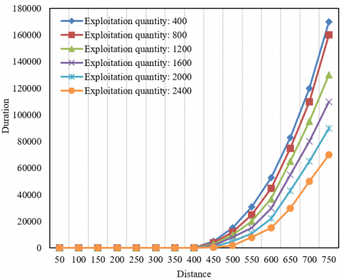
Figure 4. Curve of heat transfixion duration under different conditions
It can be seen from the Figure 4 that the greater the thickness τ of the aquifer, the greater the distance q0 between the cold- front surface of groundwater flow and the heat outlet, the smaller the water exploitation quantity E, and the longer the heat transfixion duration.
Table 1. Calculation table of average velocity of groundwater flow under different exploitation quantities
|
Exploitation quantity |
Mechanical energy difference |
Hydraulic slope |
Flow velocity |
|
2000 |
2.98 |
0.042 |
1.36 |
|
3000 |
3.62 |
0.051 |
2.35 |
|
3500 |
4.18 |
0.063 |
2.72 |
|
4500 |
6.35 |
0.084 |
3.85 |
|
5500 |
7.62 |
0.098 |
4.93 |
Under the effects of heat conduction and convection, the difference between the water temperature at the pumping and recharging ports and the initial aquifer temperature will cause heat transfixion. This paper studied the differences in the influence range of the groundwater flow temperature field under different exploitation quantities to reduce the occurrence probability or duration of heat transfixion. Table 1 shows the calculated average flow velocities of groundwater flow under different exploitation quantities. It can be seen that the greater the exploitation quantity of groundwater, the greater the hydraulic slope and seepage velocity near the heat outlet.
Considering that the temperature changes with time, Figure 5 shows the curve of groundwater temperature under different flow velocities. It can be seen that the temperature change is small when the groundwater flow seepage velocity is large, and that the temperature changes at a increasingly greater speed when the groundwater flow seepage velocity is small.
Figure 5. Curve of groundwater temperature under different flow velocities
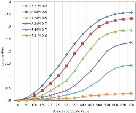
Figure 6. Curve of groundwater temperature under convective conditions
Figure 6 shows the groundwater temperature curve with only convection conditions taken into account. It can be seen that as the seepage velocity of groundwater flow decreases, the range of the temperature field affected by geothermal fluids becomes larger. When the groundwater seepage velocity is 7.84*10-6, the groundwater flow temperature field is affected by geothermal fluids by only about 0.65℃, and when the groundwater seepage velocity is reduced to 3.17*10-9, the groundwater flow temperature field is affected by geothermal fluids by around 4℃. It can be seen that the influence range is expanded.
Table 2 lists the calculation results of the mechanical energy contained by the groundwater flow per unit weight in each observation hole in a simulation cycle. Based on the calculated mechanical energy values of groundwater flow in each observation well obtained at different time points listed in the table and the observation well spacing, the hydraulic slope and groundwater level trend line can be further calculated and obtained. It can be said that, when the hydraulic slope is maintained at the same level, the geothermal flow field will tend to reach a new stable state of flow transfixion.
Table 2. Fluid energy calculation table
|
Time |
Observation hole number |
||||||
|
1 |
2 |
3 |
4 |
5 |
6 |
7 |
|
|
50h |
-18.235 |
-18.035 |
-17.821 |
-17.923 |
-17.219 |
-16.421 |
-16.159 |
|
300h |
-18.634 |
-18.176 |
-17.903 |
-17.126 |
-17.153 |
-16.532 |
-16.147 |
|
500h |
-18.326 |
-18.187 |
-17.178 |
-17.657 |
-17.436 |
-16.542 |
-16.184 |
|
800h |
-18.726 |
-18.236 |
-18.072 |
-17.270 |
-17.301 |
-16.377 |
-16.124 |
|
1000h |
-18.360 |
-18.342 |
-18.308 |
-17.154 |
-17.207 |
-16.270 |
-16.257 |
|
2000h |
-18.663 |
-18.412 |
-18.236 |
-17.287 |
-17.319 |
-16.337 |
-16.980 |
|
3000h |
-18.312 |
-18.218 |
-18.324 |
-17.213 |
-17.325 |
-16.352 |
-16.221 |
(a)
(b)
(c)
(d)
(e)
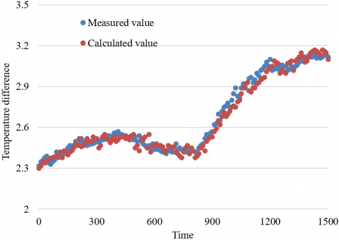
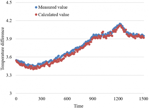
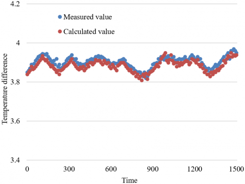
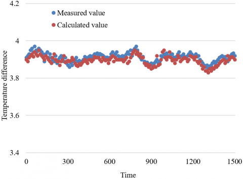
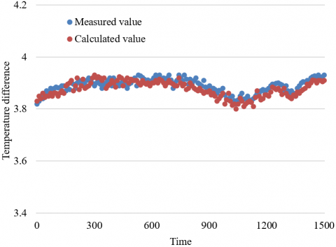
Figure 7. Time-varying curves of measured and calculated temperature differences
Figure 7 shows the time-varying curves of the temperature differences measured and calculated at each observation hole except recharge port 1 and pumping port 8. It can be seen that as the distance from the recharge port increases, the fluctuations of both the measured temperature difference and the calculated temperature difference at each observation hole gradually tend to flatten. The measured and calculated temperature differences at Observation Holes 2 and 3 near the recharging port fluctuated greatly, as shown in Figure 7(a) and (b), while those at Observation Holes 3, 4 and 5 far from the recharging port fluctuated less. The fluctuations were the smallest at Observation Hole 5, which is the closest to the pumping port. It can be clearly seen that the groundwater at this observation hole is in a stable flow state and that the temperature difference is relatively stable.
This paper analyzed and studied the influencing mechanism of geothermal fluids on the dynamic changes of groundwater flow and heat transfer temperature. First, a differential equation of heat conduction of geothermal fluids and a groundwater flow-geothermal fluids thermal coupling model were constructed to study both the seepage state and the heat transfer of groundwater flow in the energy extraction process. Then, an analytical model for the influence of groundwater seepage on heat transfixion was established, directly showing the relevant mechanism, and a water level contour map of different aquifers in the pumping and recharging process was given. Based on the experimental results, the curve of heat transfixion duration under different conditions, the curve of groundwater temperature under different flow velocities, and the curve of groundwater temperature under convective conditions were drawn, and the differences in the influence range of groundwater flow temperature field under different exploitation quantities were analyzed. Through the analysis of the time-varying curves of the measured and calculated temperature differences at the observation holes, the effectiveness of the constructed model was verified, and it was also concluded that, with the distance from the recharging port increasing, the fluctuations of both measured and calculated temperature differences at the observation holes tend to flatten.
This paper was supported by the Open Fund project of State Key Laboratory of Hydroscience and Engineering of Tsinghua University (Grant No.: sklhse-2020-A-01).
[1] Kabeyi, M.J.B., Olanrewaju, O.A. (2021). Central versus wellhead power plants in geothermal grid electricity generation. Energy, Sustainability and Society, 11(1): 7. https://doi.org/10.1186/s13705-021-00283-8
[2] Shulyupin, A.N. (2017). Steam-water flow instability in geothermal wells. International Journal of Heat and Mass Transfer, 105: 290-295. https://doi.org/10.1016/j.ijheatmasstransfer.2016.09.092
[3] Watanabe, N., Kikuchi, T., Ishibashi, T., Tsuchiya, N. (2017). ν-X-type relative permeability curves for steam-water two-phase flows in fractured geothermal reservoirs. Geothermics, 65: 269-279. https://doi.org/10.1016/j.geothermics.2016.10.005
[4] Ramazanov, M.M., Alkhasova, D.A., Abasov, G.M. (2017). Flows and heat exchange in a geothermal bed in the process of extraction of a vapor–water mixture from it. Journal of Engineering Physics and Thermophysics, 90(3): 606-614. https://doi.org/10.1007/s10891-017-1606-x
[5] Salimi, H., Groenenberg, R., Wolf, K.H. (2011). Compositional flow simulations of mixed CO2-water injection into geothermal reservoirs: Geothermal energy combined with CO2 storage. 36th Workshop on Geothermal Reservoir Engineering, Stanford University, Stanford, California, pp. 169-181.
[6] Gudjonsdottir, M., Eliasson, J., Harvey, W., Palsson, H., Saevarsdottir, G. (2010). Assessing relative permeabilities of two phase flows of water and steam in geothermal reservoirs: State of the art relations. GRC Transactions, 34: 1-9.
[7] Alkhasov, A., Bulgakova, N., Ramazanov, M. (2020). Studies of the heat and mass transfer phenomena when flowing a vapor–water mixture through the system of geothermal reservoir–well. Geomechanics and Geophysics for Geo-energy and Geo-resources, 6(1): 11. https://doi.org/10.1007/s40948-019-00132-1
[8] del Ama Gonzalo, F., Ramos, J.A.H. (2016). Testing of water flow glazing in shallow geothermal systems. Procedia Engineering, 161: 887-891. https://doi.org/10.1016/j.proeng.2016.08.742
[9] Ghasemi-Fare, O., Basu, P. (2015). Numerical modeling of thermally induced pore water flow in saturated soil surrounding geothermal piles. Geotechnical Special Publication, pp. 1668-1677. https://doi.org/10.1061/9780784479087.151
[10] Henderson Jr, H.I., Khattar, M.K., Carlson, S.W., Walburger, A.C. (2000). The implications of the measured performance of variable flow pumping systems in geothermal and water loop heat pump applications. ASHRAE Transactions, 106: 533.
[11] Becker, W., Christensen, D., Cutler, D., Maguire, J., McCabe, K., Reese, S., Speake, A. (2021). Technoeconomic design of a geothermal-enabled cold climate zero energy community. Journal of Energy Resources Technology, 143(10): 100902. https://doi.org/10.1115/1.4049456
[12] Isaji, R., Okano, O., Ohtani, T., Takagi, E., Sugihara, Y., Ueda, A. (2021). Sr isotope geochemical study of geothermal water and rocks from a newly drilled well for geothermal power generation and hot spring waters in the Okuhida Hot Spring, Gifu, Japan. Geothermics, 91: 102018. https://doi.org/10.1016/j.geothermics.2020.102018
[13] Wang, Y., Yu, L., Nazir, B., Zhang, L., Rahmani, H. (2021). Innovative geothermal-based power and cooling cogeneration system; Thermodynamic analysis and optimization. Sustainable Energy Technologies and Assessments, 44: 101070. https://doi.org/10.1016/j.seta.2021.101070
[14] Tomaszewska, B., Akkurt, G.G., Kaczmarczyk, M. et a. (2021). Utilization of renewable energy sources in desalination of geothermal water for agriculture. Desalination, 513: 115151. https://doi.org/10.1016/j.desal.2021.115151
[15] Ansari, S.A., Kazim, M., Khaliq, M.A., Ratlamwala, T.A.H. (2021). Thermal analysis of multigeneration system using geothermal energy as its main power source. International Journal of Hydrogen Energy, 46(6): 4724-4738. https://doi.org/10.1016/j.ijhydene.2020.04.171
[16] Ilko, J., Rusko, M., Halper, C., Majernik, M., Majernik, S. (2020). Flow measurement on hot water lines at geothermal power plant using ultrasonic method. Annals of DAAAM & Proceedings, 7(1): 341-347. https://doi.org/10.2507/31th.daaam.proceedings.xxx
[17] Fujii, S., Ishigami, Y., Kurihara, M. (2019). Development of geothermal reservoir simulator for predicting water-steam flow behavior considering non-equilibrium state and MINC/EDFM model. SPWLA 25th Formation Evaluation Symposium of Japan, Chiba, Japan.
[18] Phuoc, T.X., Massoudi, M., Wang, P., McKoy, M.L. (2019). Heat losses associated with the upward flow of air, water, CO2 in geothermal production wells. International Journal of Heat and Mass Transfer, 132: 249-258. https://doi.org/10.1016/j.ijheatmasstransfer.2018.11.168
[19] Shulyupin, A.N., Chermoshentseva, A.A., Varlamova, N.N. (2019). Numerical study of the stability of the steam-water flow in pipelines of geothermal gathering system. Proc. 5th Int. Conf. on Information Technologies and High-Performance Computing, Khabarovsk, Russia, pp. 103-109.
[20] Qiao, Z., Tang, Y., Zhang, L., et al. (2019). Performance analysis and optimization design of an axial-flow vane separator for supercritical CO2 (sCO2)-water mixtures from geothermal reservoirs. International Journal of Energy Research, 43(6): 2327-2342. https://doi.org/10.1002/er.4452
[21] Ovando-Chacon, S.L., Tacias-Pascacio, V.G., Ovando-Chacon, G.E., Rosales-Quintero, A., Rodriguez-Leon, A., Ruiz-Valdiviezo, V.M., Servin-Martinez, A. (2020). Characterization of thermophilic microorganisms in the geothermal water flow of El Chichón Volcano Crater Lake. Water, 12(8): 2172. https://doi.org/10.3390/w12082172
[22] Assad, M.E.H., Said, Z., Khosravi, A., Salameh, T., Albawab, M. (2019). Parametric study of geothermal parallel flow double-effect water-LiBr absorption chiller. 2019 Advances in Science and Engineering Technology International Conferences (ASET), Dubai, United Arab Emirates, pp. 1-6. https://doi.org/10.1109/ICASET.2019.8714434
[23] Kruszewski, M., Hofmann, H., Alvarez, F.G., et al. (2021). Integrated stress field estimation and implications for enhanced geothermal system development in Acoculco, Mexico. Geothermics, 89: 101931. https://doi.org/10.1016/j.geothermics.2020.101931
[24] Millstein, D., Dobson, P., Jeong, S. (2021). The potential to improve the value of US geothermal electricity generation through flexible operations. Journal of Energy Resources Technology, 143(1): 010905. https://doi.org/10.1115/1.4048520
[25] Tang, Y., Qiao, Z., Cao, Y., Si, F., Romero, C.E., Rubio-Maya, C. (2020). Numerical analysis of separation performance of an axial-flow cyclone for supercritical CO2-water separation in CO2 plume geothermal systems. Separation and Purification Technology, 248: 116999. https://doi.org/10.1016/j.seppur.2020.116999