Daniel Parenden | Peter Sahupala | Hariyanto Hariyanto*
© 2021 IIETA. This article is published by IIETA and is licensed under the CC BY 4.0 license (http://creativecommons.org/licenses/by/4.0/).
OPEN ACCESS
In summer, the utilization of solar energy can possibly satisfy the water demand. This paper examines the fluid flow in solar pump systems with solar cells. Specifically, a solar pump system model was designed and subjected to an installation test. The model consists of two solar cell units connected in series, which generate electricity and flow into the pump system. By the principles of fluid mechanics, the test results were analyzed to optimize the pump efficiency. The analysis shows that the solar cell efficiency is influenced by solar intensity, while the pump loss is maximized by fluid friction. In addition, pressure increase could affect the time of water filling; the voltage and current tend to be stable or constant.
solar, solar energy, pump, solar cell
Solar energy is an abundant and green renewable energy source. One of its applications is the photovoltaic (PV) cells, which convert solar radiation directly into electrical energy [1]. Located in the southern part of Papua Province, Indonesia, Merauke Regency (E: 137°-141°; S: 6°-9°) is known for its abundance of solar resource. It is one of the 29 regencies/cities in the southern part of that province. The regency is bordered by Boven Digoel Regency and Mappi Regency on the north, Papua New Guinea (PNG) on the east, and the Arafura Sea on the west and the south. There are strong economic ties between the regency with neighboring countries like PNG, and Australia, and the island countries in the South Pacific [2].
According to the climate data published by the Merauke Office of Meteorology and Geophysics, the wind velocity remains the same in the regency all year round. In the coastal region, the wind blows strongly at about 4-5 m/s, and the depth of wind goes around 2 m/s. The annual mean sun exposure in Merauke is 6.62h. The daily mean sun exposure stands at 5.5h in July, and peaks at 8.43h in September. The regency is quite humid, due to the tropical climate. On average, the humidity falls between 78% and 81% [3]. The natural environment of Merauke is very favorable for the development of multi-purpose solar cells [4].
In a solar pump system, PVs are usually combined with a water-producing pump. The pump operation, which is driven by the electrical energy generated by PVs, aims to suck and distribute water [5, 6]. As the fluid flows through the pipe and pump installation, energy loss inevitably occurs, which determines the energy efficiency of the solar pump system [7]. Tiwari et al. [8, 9] combined solar cells with pumps for agricultural irrigation, and discovered the following phenomena: The combined system works well in agricultural irrigation; the water yield is greatly affected by the oscillations in head pump and solar radiation. Nonetheless, they did not explain the energy loss at the pump in details.
This paper develops an analysis method for fluid mechanics. The maximum energy loss and optimal pump efficiency were determined based on the test data on solar water pump installation.
The remainder of this paper is organized as follows: Section 2 describes the properties of solar energy, solar cells, and pumps, and presents the head pump equations that computes the output power and efficiency; Section 3 introduces the research scheme, displays the test results, and carries out in-depth discussions. Section 4 concludes the research.
2.1 Solar radiation
The energy waves passing through space emit radiation of different wavelengths. Electromagnetic radiation concentrates on the wavelengths that provide lots of energy stimulation. The shorter the wavelength, the greater the energy. The radiation emitted from the solar surface varies in wavelength, ranging from the longest radio waves to the shortest X-rays and gamma rays.
In 1997, the Solar Energy Panel of National Aeronautics and Space Administration (NASA) classified new energy collection systems into two categories, namely, natural collection systems, and technological collection systems. The former systems acquire energy from water, wind, organic fuel, and sea temperature gradient; the latter systems collect power through PV power generation, and thermal heat generation.
The PVs convert solar radiation into electrical energy. Solar radiation also produces thermal energy, which is commonly concentrated by collectors, and utilized by solar collectors, heat pumps, etc. [10].
The intensity of solar radiation is reduced by absorption and reflection by the air, immediately before the sunrays reaching the earth’s surface. In the atmosphere, ozone absorbs the radiation with short wavelengths (ultraviolet), while carbon dioxide and water vapor absorb the radiation with longer wavelengths (infrared). Apart from the reduction of direct earth radiation (headlights) through absorption, radiations from gas, dust, and water vapor molecules are also emitted in the air [11].
2.2 Solar cell
Solar cells generate electrical energy by the PV effect on semiconductors. A solar cell typically consists of two ultrathin semiconductor plates, which are often combined into one plate of negative (n)-semiconductors and positive (p)-semiconductors. The p-semiconductor plate is arranged above the n-semiconductor plate. The p-semiconductors (charge: +) are porous instruments made of boron-doped silicon, while the n-semiconductors (charge: -) are electron-rich instruments made of phosphorus-doped silicon. The boron and phosphorus deliver an excess of free electrons.
The basis of solar cells is extra small pieces of silicon, which are coated with special chemicals. In general, solar cells are at least 0.3 mm in thickness, and prepared from cut semiconductor material with positive and negative poles. It is the active elements (semiconductors) in the cells that convert solar energy into electrical energy, using the PV effect.
When a solar cell is exposed to sunlight, each n-semiconductor serves as a negatively charged electrode, while each p-semiconductor acts as a positively charged electrode. The two electrodes have a potential difference. If they are connected by a wire, an electrical current will occur from the electrode (+) to the electrode (-) [12]. Figure 1 is the sketch map of a solar cell.
Figure 1. Sketch map of a solar cell
Under the direct sunlight of 1,000 W/m2 and temperature of 25℃, a solar cell can generate a direct current (DC) of 20-40 mA/cm2 and a voltage of 0.7-0.85 V. Depending on the material, the area of a solar cell ranges between 1 cm2 and 4 cm2. To produce more electrical energy (i.e., higher current and voltage), several solar cells are often connected in series and in parallel to form a module. Sometimes, multiple such modules are integrated into a solar cell panel.
2.3 Centrifugal pump
The pump moves fluid to a higher location by increasing fluid pressure. The increased fluid pressure aims to overcome the drainage barriers, which take the form of pressure difference, height, or friction barrier.
The centrifugal force arises as an object moves along a curved (circular path). Therefore, a centrifugal pump is a dynamic working pump that uses a rotating impeller to increase the fluid pressure [6].
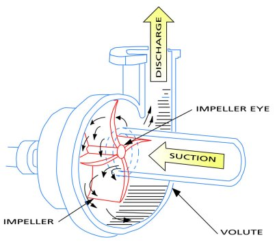
Centrifugal pumps are driven by motors. The power from the motor is transferred to the pump shaft to rotate the impeller attached to the shaft. Once the impeller rotates, the fluid is sucked through the eye on the veil into the impeller. Under the impulse of the blades, the fluid within the impeller also rotates on the impeller due to the centrifugal force. The working principle of a centrifugal pump is explained in Figure 2.
Figure 2. The working principle of a centrifugal pump
Since the rotating impeller creates a centrifugal force, the fluid flows from the center of the impeller to the outside of blades through the channel between the blades, and leaves the impeller at a high velocity. As the fluid picks up speed, its pressure head increases, so does the head velocity. The fast fluid leaving the impeller than passes through an expansion channel, forming a spiral around the impeller, and is directed through a nozzle to the outside of the pump.
The capacity generated by a centrifugal pump is proportional to the rotation velocity, while the total height (pressure) generated by the pump is proportional to the square of the velocity.
2.4 Head pump
The head pump refers to the amount of energy needed by the pump to change the fluid from the initial state to the planned final state according to the conditions of the pump installation. It is generally expressed in units of length. Pump head can also be interpreted as the energy supplied by the pump into the fluid in the form of high pressure. The compressive height is defined as the height that the fluid must reach to obtain the same amount of energy as that contained in a unit of fluid weight under the same conditions. Owing to the conservation of energy, the shape of the head (height) can vary from cross-section to cross-section. But in reality, there are always energy losses known as head losses (hL) [9].
2.4.1 Head mayor losses
Major loss is the energy loss induced by the friction between the fluid flow and the pipe wall. The magnitude of the loss hinges on the pipe length. The major loss hL(m) along a pipe can be calculated by:
${{h}_{L}}\,=\,f\frac{L}{D}\frac{{{V}^{2}}}{2g}$ (1)
where, f is the friction factor; V is the mean velocity of the fluid in the pipe (m/s); D is the pipe diameter (m). The value of f can be obtained from the Moody diagram as a function of the Reynolds number, and the relative or equivalent roughness (relative roughness - ε / D). From the Moody diagram, the relative roughness can be viewed as a function of the nominal pipe diameter and surface roughness of the pipe (ε), which depends on the pipe material. The Moody diagram equation can be expressed as [13]:
$f\bigcirc \left( \operatorname{Re},\frac{\varepsilon }{D} \right)$ (2)
The magnitude of the Reynolds number depends on the type of flow in the pipe, which is either laminar or turbulent. The flow in the pipe is greatly affected by velocity, kinematic viscosity, or the fluid type, which is in turn influenced by pipe diameter. To determine the type of flow in the pipe, the Reynolds number must be computed first by:
$\operatorname{Re}=\frac{VD}{\nu }$ (3)
where, ν is the kinematic viscosity of the fluid (m2/s):
$\nu =\frac{\mu }{\rho }$ (4)
so that,
$\operatorname{Re}=\frac{\rho VD}{\mu }$ (5)
where, Re is the Reynolds number; ρ is the fluid density (kg/m3); V is the mean flow velocity (m/s); D is the pipe diameter (m); μ is the dynamic viscosity of the fluid (N·s/m2). If the fluid is a laminar flow (Re < 2,300), the friction factor (f) can be calculated by:
$f=\frac{64}{\operatorname{Re}}$ (6)
If the fluid is a turbulent flow (Re > 4,000), the friction factor (f) can be obtained with the Moody diagram as described above. I Re = 2,300-4,000, the flow must be a transition flow.
2.4.2 Minor head loss
Minor head loss is the head loss of fittings or pipe connections (e.g., valves, elbows, strainers, and connections), the loss at the inlet, the loss at the outlet, the loss in pipe expansion or contraction segment throughout the pipe network. The minor head loss can be calculated by:
${{h}_{f}}=k\frac{{{V}^{2}}}{2g}$ (7)
where, hf is the head loss (m); k is the friction factor of the fittings or pipe connections; V is the mean flow velocity (m/s).
The losses of fittings or pipe connections can be obtained by looking up the tables, where the values are presented as the equivalent length of a straight pipe. The total loss of the pipe network can be expressed as:
${{h}_{tot}}={{h}_{L}}+{{h}_{f}}$ (8)
where, htot is the total losses (m); hf is the number of minor losses (m).
2.4.3 Power of centrifugal pump
The input power of a centrifugal pump can be defined as the product of voltage and current to the pump motor:
${{P}_{inM}}=V\text{ x }I$ (8)
where, V is the voltage (V); I is the current (A).
The output power of the pump refers to the energy effectively received by the water from the pump. It is commonly called hydraulic fluid power. The output power can be calculated by:
${{P}_{f}}=\rho \text{ x }g\text{ x }Q\text{ x }H$ (10)
where, Pf is the pump output power (W); ρ is the water density (kg/m3); g is the acceleration of gravity (m/s2); Q is the water discharge; H is the head (m).
The head has an impact on the size of the pump and driver. The head of a pump is the pressure difference (fluid height) between the inlet and outlet.
2.4.4 Pump efficiency
The pump efficiency ηp is a comparison between pump output power and pump input power:
${{\eta }_{p}}=\frac{{{P}_{f}}}{{{P}_{inM}}}\text{x 100 }\!\!%\!\!\text{ }$ (11)
2.5 DC motor
DC motor converts DC electrical energy into mechanical energy via rotation. Physically, a typical DC motor encompasses a stationary part (stator) and a rotating part (rotor). The DC motor works by the principle of interaction between two magnetic fluxes: the north-south magnetic flux produced by the field coil, and the circular magnetic flux produced by the anchor coil. The interaction between the two magnetic fluxes creates a force that will cause torsional or torsional moments. Hence, a solar cell is essentially a large photodiode. Referring to the PV phenomenon, the solar cell is designed in such a way that it can produce as much power as possible.
In the solar cell, the p-semiconductors form an ultrathin surface layer, through which the sunlight can directly penetrate to the junction. This p-section is coated with a ring-shaped nickel layer, providing a positive output terminal. Under the P section, there is an n- section coated with nickel as well, working as a negative output terminal. Lots of solar cells are needed to generate a sufficiently large power. Usually, these cells are arranged into large PV panels.
3.1 Test scheme
This paper designs a model for installation test in the mechanical engineering laboratory at Universitas Musamus, Indonesia. The test was carried out in the following steps: prepare research tools and materials; design a solar pump installation in a DC motor rotation system; assemble a solar pump motor, install a solar water pump, and carry out the isntallation test. After collecting suffient test data, the authors performed an in-depth analysis.
3.2 Data analysis
The fluid mechanics of pumps and pump systems were conisdered in the data analysis to optimize the pump efficiency. Table 1 lists the installation test data on the solar water pump with battery installed in series, without charging the solar module.
Table 1. Test parameters
|
Test parameters |
Head 2 Meters |
Head 3 Meters |
Head 4 Meters |
|
Solar panel voltage |
24.01 V |
24.31 V |
24.39 V |
|
Solar panel current |
32 A |
31 A |
32 A |
|
Area of 1 solar cell panel |
784x50x5x35 |
784x50x5x35 |
784x50x5x35 |
|
DC motor voltage |
24 V |
24 V |
24 V |
|
Water density at 35℃ |
995.68 kg/m3 |
995.68 kg/m3 |
995.68 kg/m3 |
|
Inner pipe diameter |
0.026 m |
0.026 m |
0.026 m |
|
Earth’s gravity |
9.81 m/s |
9.81 m/s |
9.81 m/s |
|
Water discharge |
5 litter |
5 litter |
5 litter |
|
Time |
15.31 s |
15.31 s |
15.31 s |
|
Suction pipe length |
4 m |
4 m |
4 m |
Table 2. Calculation results of solar water pump installation
|
Measured data |
Head 2 meters |
Head 3 meters |
Head 4 meters |
|
Fluid flow velocity |
0.31 m3/s |
0.35 m3/s |
0.36 m3/s |
|
Friction-induced fluid flow loss |
0 m/s |
0 m/s |
0 m/s |
|
Water viscosity at 35℃ |
11.210 |
12.692 |
13.018 |
|
Fluid flow loss (bent 90°) |
0.00039 m |
0.005 m |
0.00052 m |
|
Fluid flow loss (straight connection) |
0.00124 |
0.002 m |
0.00019 m |
|
Total head |
4.00514 m |
4.007 m |
4.0109 m |
|
Hydraulic fluid power |
6.25 W |
8.48 W |
10.53 W |
|
Pump efficiency |
0.82% |
1.12% |
1.31% |
Table 2 shows the calculation results of the solar power pump system at different head heights. When the pump ran at 24.01 V and 32 A, the delivery head was increased by 2m, and the water discharge was 5L in 15.31s. When the pump ran at 24.31 V and 31 A, the delivery head increased by 3m, and the water discharge was 5L in 17.22s. When the pump ran at 24.39 V and 32 A, the delivery head increased by 4m, and the water discharge was 5L in 18.11s. During night operations, the pump could operate for 2h50min with a head of 4m; the remaining power of the battery was 11.56 V and 15 A, and the initial power was 20.50 V and 32 A.
Through the above analysis, it is learned that the installation of solar pumps with different delivery heights results in a maximum hydraulic fluid output of 10.5 W with an efficiency of 1.31%. The power and efficiency are influenced by solar intensity, which generates currents and voltages in the solar cell. Meanwhile, the maximum fluid loss induced by friction at the pump was zero; the fluid losses at an inclination of 90° and in the straight connection were 0.00052 and 0.00019, respectively; the total height peaked at 4.0109m. Therefore, increasing the head can affect charging time and water output, while voltage and current tend to be stable or constant. The above results can be adopted to develop solar panels of other materials and models of different pump installations, and determine the optimal ratio of output power to maximum efficiency.
Thank you to the research team at the Laboratory of the Department of Mechanical Engineering, Faculty of Engineering, Universitas Musamus for helping with research and installation of equipment during testing.
|
hL |
mayor losses, m |
|
hf |
minor losses, m |
|
htot |
total losses, m |
|
f |
friction factor |
|
V |
the average velocity of liquid in a pipe, m.s-1 |
|
D |
the inner diameter of the pipe, m |
|
Re |
Reynold Number |
|
k |
coefficient of friction in the fitting |
|
g |
acceleration due to gravity, m.s-2 |
|
PinM |
input power, W |
|
Pf |
output power, W |
|
ηp |
pump efficiency, % |
|
V |
voltage, V |
|
I |
current, A |
|
Q |
water discharge, m3 |
|
H |
head, m |
|
Greek symbols |
|
|
ε |
surface roughness in the pipe, m |
|
ν |
kinematic viscosity of liquid, m2.s-1 |
|
μ |
dynamic viscosity in liquids, liquids N-s.m-2 |
|
ρ |
liquid density, kg.m-3 |
[1] Messenger, R., Abtahi, H.A. (2018). Photovoltaic Systems Engineering. CRCPres. Taylor & Francis Goup. London New York.
[2] Statistics Data Data. Regency Merauke in figures. Indonesian.https://meraukekab.bps.go.id/publication/2018/08/20/068d3eb8ce3a1b4d204b6b05/kabupaten-merauke-dalam-angka-2018.html, accesed on Jan. 13, 2020.
[3] BMKG. Meteorology Climatology and Geophysics Council. Indonesian. https://www.bmkg.go.id/cuaca/prakiraan cuaca.bmkg?Kota=Merauke&AreaID=501450&Prov=24, accesed on Jan. 20, 2020.
[4] Hariyanto, H., Parenden, D., Vincēviča-Gaile, Z., Adinurani, P.G. (2020). Potential of new and renewable energy in merauke regency as the future energy. E3S Web of Conferences, 190: 00012. https://doi.org/10.1051/e3sconf/202019000012
[5] Chandel, S.S., Naik, M.N., Chandel, R. (2015). Review of solar photovoltaic water pumping system technology for irrigation and community drinking water supplies. Renewble Sustainable Energy Review, 49: 1084-1099. http://dx.doi.org/10.1016/j.rser.2015.04.083
[6] Li, G., Jin, Y., Akram, M.W., Chen, X. (2017). Research and current status of the solar photovoltaic water pumping system – a review. Renewble Sustainable Energy Review, 79: 440-458. http://dx.doi.org/10.1016/j.rser.2017.05.055
[7] Munson, B.R., Young, D.F., Okiishi T.H. (1994). Fundamental of Fluid Mechanics, USA.
[8] Tiwari, A.K., Kalamkar, V.R. (2016). Performance investigations of solar water pumping system using helical pump under the outdoor condition of Nagpur, India. Renewable Energy, 97(9): 737-745. http://dx.doi.org/10.1016/j.renene.2016.06.021
[9] Tiwari, A.K., Kalamkar, V.R. (2018). Effects of total head and solar radiation on the performance of solar water pumping system. Renewable Energy, 118(9): 919-927. https://doi.org/10.1016/j.renene.2017.11.004 2018
[10] Pavlovic, T. (2020). The Sun and Photovoltaic Technologies. Springer Nature Switzerland AG. https://doi.org/10.1007/978-3-030-22403-5
[11] Kalogirou, S.A. (2009). Solar Energy Engineering: Processes and Systems, USA.
[12] Radziemska, E. (2009). Performance analysis of a photovoltaic-thermal integrated system. International Journal Photoenergy, 732093(6). https://doi.org/10.1155/2009/732093
[13] White, F.M. (2009). Fluid Mechanics. University of Rhode Island, McGraw-Hill, New York.