Avula Benerji Babu* | Gundlapally Shiva Kumar Reddy | Nilam Venkata Koteswararao
© 2021 IIETA. This article is published by IIETA and is licensed under the CC BY 4.0 license (http://creativecommons.org/licenses/by/4.0/).
OPEN ACCESS
In the present paper, linear and weakly nonlinear analysis of magnetoconvection in a rotating fluid due to the vertical magnetic field and the vertical axis of rotation are presented. For linear stability analysis, the normal mode analysis is utilized to find the Rayleigh number which is the function of Taylor number, Magnetic Prandtl number, Thermal Prandtl number and Chandrasekhar number. Also, the correlation between the Rayleigh number and wave number is graphically analyzed. The parameter regimes for the existence of pitchfork, Takens-Bogdanov and Hopf bifurcations are reported. Small-amplitude modulation is considered to derive the Newell-Whitehead-Segel equation and using its phase-winding solution, the conditions for the occurrence of Eckhaus and zigzag secondary instabilities are obtained. The system of coupled Landau-Ginzburg equations is derived. The travelling wave and standing wave solutions for the Newell-Whitehead-Segel equation are also presented. For, standing waves and travelling waves, the stability regions are identified.
bifurcation points, secondary instabilities, heat transport, travelling and standing waves
Double Diffusive convection is the process of mixing driven by the interaction of two fluid components. This can occur if the fluid consists of two or more constituents with disparate molecular diffusivity and they must contribute rival to the vertical density gradient [1]. The Double Diffusive convection problem has attracted considerable interest in the last few decades because of its wide range of applications, such as the disposal of waste material, groundwater contamination, chemical transport in packed-bed reactors, food processing and many other engineering applications. Double Diffusive convection is involved in the migration of moisture like transport in environment, magmas, groundwater and in fibrous insulation. The examples of Double Diffusive convection are magnetoconvection, Convection in Earth’s core and thermohaline convection [2].
The study of a magnetic field in a rotating fluid is more interesting in geophysics; Particularly in the research of Earth’s core. Convection in Earth’s outer core is strenuously affected by magnetic and rotational field. Drazin and Reid [3] had examined both experimental and theoretical results on thermal convection in a fluid layer in the presence and absence of a magnetic and rotational fields. The earliest work on magnetoconvection in rotating fluid was carried out by Eltayeb [4], Jones and Roberts [5, 6], Soward [7] and Tagare et al. [8]. Babu et al. [9, 10] had thoroughly investigated the nonlinear convection in the absence and presence of rotation and magnetic fields.
The number of components which must be varied for the bifurcation to occur is known as co dimension of a bifurcation. Pitchfork, Hopf, Takens-Bogdanov, Co dimension two bifurcation have been studied by Babu et al. [9, 10]. Ravi et al. [11] had investigated the stability properties of non-linear plane wave solutions of the form w=W(z)eiqx+pt. The stability of these solutions has been investigated for both real and complex Landau-Ginzburg equations by using Multiscale analysis [12].
Skew-Varicose, Eckhaus and Zigzag instabilities are examples of long wavelength instabilities. These instabilities, originally identified in the stability theory for convection rolls. These instabilities can arise may be either in stationary convection or oscillatory convection. The Eckhaus instability is an important mechanism which can lead to a considerable change in the wave number. Zigzag instability is the most unstable instability.
Hopf bifurcation gives rise to Standing waves and Travelling waves when the Rayleigh number is increased [13]. Steady state convection can take place at large Rayleigh number. In the case of weak magnetic field Standing waves are stable and for stronger fields Travelling waves are stable [14]. In case of the rotating field, either Standing and Travelling waves are stable, based on the rate of rotation and Prandtl number [15-17].
In the present paper, nonlinear magneto convection in a rotating fluid due to vertical magnetic field and vertical axis of rotation is analyzed. Basic equations for the system, linear stability analysis, two-dimensional amplitude equation, occurrence of secondary instabilities and the transport of heat by convection through Nusselt number are discussed in subsequent sections. The system of nonlinear one-dimensional amplitude equations, Benjamin-Feir instability for Standing and Travelling waves are also examined.
Let us assume that an electrically and thermally conducting fluid confined between two infinite horizontal planes of depth d with adverse temperature gradients, which is kept rotating at a constant angular velocity Ω with uniform magnetic field Ho in the z-direction. The magnetic field $\overline{H}({{H}_{x}},{{H}_{y}},{{H}_{z}})$, velocity $\overline{V}(u,v,w)$, pressure P, temperature θ, time t are non-dimensionalized by scales $k{{H}_{0}}/\eta , k/d, \mu k/{{d}^{2}}, $ ${\beta }'d$ and d2/k. Here k is the coefficient of thermal diffusivity, η is electrical resistivity, β is the adverse temperature gradient and μ is viscosity.
The dimensionless equations for the chosen system in the Boussinesq approximation are:
$\nabla .\overline{V}=0, \nabla .\overline{H}=0$ (1)
$\begin{align} & \frac{1}{{{\sigma }_{1}}}\left[ \frac{\partial \overline{V}}{\partial t}+(\overline{V}.\nabla )\overline{V} \right]-Q\frac{{{\sigma }_{2}}}{{{\sigma }_{1}}}(\overline{H}.\nabla )\overline{H}-Q\frac{\partial \overline{H}}{\partial z} \\ & =-\nabla (P+\frac{1}{2}Q\frac{{{\sigma }_{2}}}{{{\sigma }_{1}}}|H{{|}^{2}}+Q{{H}_{z}}-\frac{Ta{{\sigma }_{1}}}{8}|{{{\hat{e}}}_{z}}\times \overline{r}{{|}^{2}}) \\ & +T{{a}^{\frac{1}{2}}}(\overline{V}\times {{{\hat{e}}}_{z}})+{{\nabla }^{2}}\overline{V}+R\theta {{{\hat{e}}}_{z}}, \\\end{align}$ (2)
$\frac{\partial \theta }{\partial t}+(\overline{V}.\nabla )\theta =\omega +{{\nabla }^{2}}\theta ,$ (3)
$\frac{{{\sigma }_{2}}}{{{\sigma }_{1}}}\frac{\partial \overline{H}}{\partial t}-\frac{{{\sigma }_{2}}}{{{\sigma }_{1}}}\nabla \times (\overline{V}\times \overline{H})=\nabla \times (\overline{V}\times {{\hat{e}}_{z}})+{{\nabla }^{2}}\overline{H}.$ (4)
where, ${{\hat{e}}_{z}}$ is the unit vector along the rotational axis.
The Non-dimensional numbers $R,Q,Ta,{{\sigma }_{1}}$ and ${{\sigma }_{2}}$ are given by:
$\begin{align} & R=\frac{\alpha g{\beta }'{{d}^{4}}}{\nu k}, Q=\frac{{{\mu }_{m}}H_{0}^{2}{{d}^{2}}}{4\pi {{\rho }_{0}}\nu \eta }, Ta=\frac{4{{\Omega }^{2}}{{d}^{4}}}{{{\nu }^{2}}}, \\ & {{\sigma }_{1}}=\nu /k, {{\sigma }_{2}}=\nu /\eta . \\\end{align}$
Here R is Rayleigh number, Q is Chandrasekhar number, Ta is Taylor number, ${{\sigma }_{1}}$ is Thermal Prandtl number, ${{\sigma }_{2}}$ is Magnetic Prandtl number, ${{\rho }_{0}}$ is density, ${{\mu }_{m}}$ is Magnetic permiability, g is acceleration due to gravity.
The z-components of curl(2), of curl2(2), of curl (4) and of (4) itself, we get:
$\left( \frac{1}{{{\sigma }_{1}}}\frac{\partial }{\partial t}-{{\nabla }^{2}} \right)\xi -Q\frac{\partial {{J}_{z}}}{\partial z}-T{{a}^{1/2}}\frac{\partial w}{\partial z}$
$={{\hat{e}}_{z}}.\{-\frac{1}{{{\sigma }_{1}}}\left[ \nabla \times \left( \overline{V}.\nabla \right)\overline{V} \right]+Q\frac{{{\sigma }_{2}}}{{{\sigma }_{1}}}\left[ \nabla \times \left( \overline{H}.\nabla \right)\overline{H} \right]\},$
$\left( \frac{1}{{{\sigma }_{1}}}\frac{\partial }{\partial t}-{{\nabla }^{2}} \right){{\nabla }^{2}}w-Q\frac{\partial }{\partial z}{{\nabla }^{2}}{{H}_{z}}-R\nabla _{h}^{2}\theta +T{{a}^{1/2}}\frac{\partial \xi }{\partial z}$ (5)
$={{\hat{e}}_{z}}.\{\frac{1}{{{\sigma }_{1}}}\left[ \nabla \times \nabla \times \left( \overline{V}.\nabla \right)\overline{V} \right]-Q\frac{{{\sigma }_{2}}}{{{\sigma }_{1}}}[\nabla \times \nabla \times (\bar{H}\cdot \nabla )\bar{H}]\},$
$\left( \frac{{{\sigma }_{2}}}{{{\sigma }_{1}}}\frac{\partial }{\partial t}-{{\nabla }^{2}} \right){{J}_{z}}-\frac{\partial \xi }{\partial z}={{\hat{e}}_{z}}\cdot \{\frac{{{\sigma }_{2}}}{{{\sigma }_{1}}}\left[ \nabla \times \nabla \times \left( \overline{V}.\nabla \right)\overline{V} \right]\},$
$\left( \frac{{{\sigma }_{2}}}{{{\sigma }_{1}}}\frac{\partial }{\partial t}-{{\nabla }^{2}} \right){{H}_{z}}-\frac{\partial \xi }{\partial z}={{\hat{e}}_{z}}.\{\frac{{{\sigma }_{2}}}{{{\sigma }_{1}}}\left[ \nabla \times \left( \overline{V}.\nabla \right)\overline{V} \right]\}.$
Here ${{H}_{z}}={{\hat{e}}_{z}}.\overline{H}, {{J}_{z}}={{\hat{e}}_{z}}.\left( \nabla \times \overline{H} \right)$ and $\xi ={{\hat{e}}_{z}}.\left( \nabla \times \overline{V} \right)$. Now eliminating $\theta , {{H}_{z}},\xi ,{{J}_{z}}$from the relation (5) and together with (3), we get:
$Lw=N.$ (6)
where,
$\begin{align} & L=D{{\nabla }^{2}}{{\left( {{D}_{{{\sigma }_{1}}}}{{D}_{{{\sigma }_{2}}}}-Q\frac{{{\partial }^{2}}}{\partial {{z}^{2}}} \right)}^{2}} \\ & -\left( {{D}_{{{\sigma }_{1}}}}{{D}_{{{\sigma }_{2}}}}-Q\frac{{{\partial }^{2}}}{\partial {{z}^{2}}} \right)R{{D}_{{{\sigma }_{2}}}}\nabla _{h}^{2}+TaDD_{{{\sigma }_{2}}}^{2}\frac{{{\partial }^{2}}}{\partial {{z}^{2}}}, \\\end{align}$ (7)
$\begin{align} & N= \\ & \left( {{D}_{{{\sigma }_{1}}}}{{D}_{{{\sigma }_{2}}}}-Q\frac{{{\partial }^{2}}}{\partial {{z}^{2}}} \right)[D{{D}_{{{\sigma }_{2}}}}{{{\hat{e}}}_{z}}.[\frac{1}{{{\sigma }_{1}}}\left( \nabla \times \nabla \times (\overline{V}.\nabla )\overline{V} \right) \\\end{align}$
$-Q\frac{{{\sigma }_{2}}}{{{\sigma }_{1}}}(\nabla \times \nabla \times (\overline{H}.\nabla )\overline{H})]-{{D}_{{{\sigma }_{2}}}}R\nabla _{h}^{2}(\overline{V}.\nabla )\theta $
$+Q{{\nabla }^{2}}D\frac{\partial }{\partial z}{{\hat{e}}_{z}}.\frac{{{\sigma }_{2}}}{{{\sigma }_{1}}}\left( \nabla \times (\overline{V}\times \overline{H}) \right)]$ (8)
$-T{{a}^{1/2}}{{D}_{{{\sigma }_{1}}}}{{D}_{{{\sigma }_{2}}}}\frac{\partial }{\partial z}[{{D}_{{{\sigma }_{2}}}}{{\hat{e}}_{z}}.\left( -\frac{1}{{{\sigma }_{1}}}\left( \nabla \times (\overline{V}.\nabla )\overline{V} \right) \right.$
$\left. +Q\frac{{{\sigma }_{2}}}{{{\sigma }_{1}}}\left( \nabla \times (\overline{H}.\nabla )\overline{H} \right) \right)+Q\frac{\partial }{\partial z}{{\hat{e}}_{z}}.\left( \nabla \times \nabla \times (\overline{V}\times \overline{H}) \right)].$
where, $D=(\frac{\partial }{\partial t}-{{\nabla }^{2}})$, ${{D}_{{{\sigma }_{1}}}}=(\frac{1}{{{\sigma }_{1}}}\frac{\partial }{\partial t}-{{\nabla }^{2}})$, ${{D}_{{{\sigma }_{2}}}}=(\frac{{{\sigma }_{2}}}{{{\sigma }_{1}}}\frac{\partial }{\partial t}-{{\nabla }^{2}})$,${{\nabla }^{2}}=\left( \frac{{{\partial }^{2}}}{\partial {{x}^{2}}}+\frac{{{\partial }^{2}}}{\partial {{y}^{2}}}+\frac{{{\partial }^{2}}}{\partial {{z}^{2}}} \right)$ and $\nabla _{h}^{2}=\left( \frac{{{\partial }^{2}}}{\partial {{x}^{2}}}+\frac{{{\partial }^{2}}}{\partial {{y}^{2}}} \right)$.
2.1 Boundary conditions
The fluid is bounded by the planes z=0 and z=1. For further analysis free-free boundary conditions are considered. Hence
$\theta=0, w=0, \frac{\partial w_{z}}{\partial z}=0 \text { and } \frac{\partial^{2} w}{\partial z^{2}}=0 \text { on } z=0, z=1 \forall x, y$.
For the linear stability analysis substitute w=W(z)ei(lx+my)+pt in Lw=0, which is a linearized version of the Eq. (6), hence
$\begin{align} & [\left( p-\left( {{D}^{2}}-{{q}^{2}} \right) \right)\left( {{D}^{2}}-{{q}^{2}} \right) \\ & {{[\left( \frac{{{\sigma }_{2}}}{{{\sigma }_{1}}}p-\left( {{D}^{2}}-{{q}^{2}} \right) \right)\left( \frac{1}{{{\sigma }_{1}}}p-\left( {{D}^{2}}-{{q}^{2}} \right) \right)-Q{{D}^{2}}]}^{2}} \\ & +Ta{{D}^{2}}\left( p-\left( {{D}^{2}}-{{q}^{2}} \right) \right){{\left( \frac{{{\sigma }_{2}}}{{{\sigma }_{1}}}p-\left( {{D}^{2}}-{{q}^{2}} \right) \right)}^{2}} \\ & +Ta{{D}^{2}}\left( p-\left( {{D}^{2}}-{{q}^{2}} \right) \right){{\left( \frac{{{\sigma }_{2}}}{{{\sigma }_{1}}}p-\left( {{D}^{2}}-{{q}^{2}} \right) \right)}^{2}} \\\end{align}$
$\begin{align} & +R{{q}^{2}}(\frac{{{\sigma }_{2}}}{{{\sigma }_{1}}}p-\left( {{D}^{2}}-{{q}^{2}} \right)) \\ & [\left( \frac{{{\sigma }_{2}}}{{{\sigma }_{1}}}p-\left( {{D}^{2}}-{{q}^{2}} \right) \right)\left( \frac{1}{{{\sigma }_{1}}}p-\left( {{D}^{2}}-{{q}^{2}} \right) \right)-Q{{D}^{2}}]]W(z)=0. \\\end{align}$ (9)
where, $D=\frac{\partial }{\partial z}$, q2=l2+m2 and p is the growth rate of the disturbances. Substituting p=iω and W(z)=sinπz in to Eq. (9), we get
$R=\frac{{{k}_{1}}{{\omega }^{8}}+{{k}_{2}}{{\omega }^{6}}+{{k}_{3}}{{\omega }^{4}}+{{k}_{4}}{{\omega }^{2}}+{{k}_{5}}+i\omega \left( {{k}_{6}}{{\omega }^{6}}+{{k}_{7}}{{\omega }^{4}}+{{k}_{8}}{{\omega }^{2}}+{{k}_{9}} \right)}{{{q}^{2}}\left( {{k}_{10}}{{\omega }^{6}}+{{k}_{11}}{{\omega }^{4}}+{{k}_{12}}{{\omega }^{2}}+{{k}_{13}} \right)},$ (10)
3.1 Stationary convection (ω=0)
For stationary convection substitute ω=0 in to Eq. (10),
${{R}_{s}}=\frac{\delta _{s}^{2}}{q_{s}^{2}}\left[ \delta _{s}^{4}+Q{{\pi }^{2}}+\frac{Ta{{\pi }^{2}}\delta _{s}^{2}}{\delta _{s}^{4}+Q{{\pi }^{2}}} \right],$ (11)
where, $q_{s}^{2}=l_{s}^{2}+m_{s}^{2}$and $\delta _{s}^{2}={{\pi }^{2}}+q_{s}^{2}$. The Rayleigh number RS represents the stationary convection of Rayleigh number R. The critical value of RS exists for qsc, where
$\begin{align} & \delta _{sc}^{6}-3q_{sc}^{2}\delta _{sc}^{4}+Q{{\pi }^{4}} \\ & +\frac{Ta{{\pi }^{2}}\delta _{sc}^{2}}{\delta _{sc}^{4}+Q{{\pi }^{2}}}\left[ {{\pi }^{2}}-q_{sc}^{2}+\frac{2q_{sc}^{2}\delta _{sc}^{4}}{\delta _{sc}^{4}+Q{{\pi }^{2}}} \right]=0, \\\end{align}$ (12)
where, $q_{sc}^{2}=l_{sc}^{2}+m_{sc}^{2}$and $\delta _{sc}^{2}={{\pi }^{2}}+q_{sc}^{2}$ From Eq. (11) q=qsc. Therefore
${{R}_{sc}}=\frac{\delta _{sc}^{2}}{q_{sc}^{2}}\left[ \delta _{sc}^{4}+Q{{\pi }^{2}}+\frac{Ta{{\pi }^{2}}\delta _{sc}^{2}}{\delta _{sc}^{4}+Q{{\pi }^{2}}} \right].$ (13)
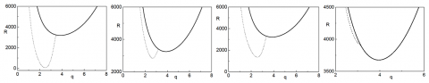
Figure 1. Marginal stability curves (Solid lines represents stationary convection and dotted lines represents oscillatory convection) Ta=1000,${{\sigma }_{1}}=1.7$,${{\sigma }_{2}}=0.5$, (a)Q=118, (b)Q=120, (c)Q=121, (d)Q=122
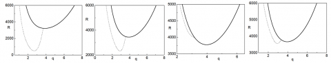
Figure 2. Marginal stability curves (Solid lines represents stationary convection and dotted lines represents oscillatory convection)$Q=120$,${{\sigma }_{1}}=1.8$,${{\sigma }_{2}}=0.5$,$(a)Ta=1000$,$(b)Ta=2000$,$(c)Ta=3000$,$(d)Ta=3500$
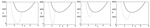
Figure 3. Marginal stability curves (Solid lines represents stationary convection and dotted lines represents oscillatory convection)$Q=120, Ta=1000, {{\sigma }_{2}}=0.5$,$(a){{\sigma }_{1}}=1.42$,$(b){{\sigma }_{1}}=1.56$,$(c){{\sigma }_{1}}=1.70$,$(d){{\sigma }_{1}}=1.85$
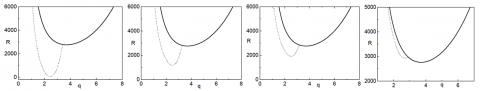
Figure 4. Marginal stability curves (Solid lines represents stationary convection and dotted lines represents oscillatory convection)$Q=90, Ta=1000, {{\sigma }_{1}}=1.8$,$(a){{\sigma }_{2}}=0.5350$,$(b){{\sigma }_{2}}=0.5375$,$(c){{\sigma }_{2}}=0.5390$,$(d){{\sigma }_{2}}=0.5410$
3.2 Oscillatory convection (ω2=0)
For Oscillatory convection $\omega \ne 0$, the Eq. (10) is complex. The Rayleigh number is always real so that equate imaginary part to zero. i.e.
${{k}_{6}}{{\omega }^{6}}+{{k}_{7}}{{\omega }^{4}}+{{k}_{8}}{{\omega }^{2}}+{{k}_{9}}=0,$ (14)
where, k6, k7, k8 and k9 are given by relation (7). We get k6>0, k7<0, k8>0 and k9>0 for $1<{{\sigma }_{2}}<{{\sigma }_{1}}$ or ${{\sigma }_{2}}<{{\sigma }_{1}}<1$ and for some values of other physical components. So by Descarte’s rule there exist at least two positive roots of Eq. (14). From k9=0, we get
$\begin{align} & Ta{{s}_{3}}{{\pi }^{2}}{{\delta }^{6}}-{{Q}^{2}}{{s}_{3}}{{\delta }^{4}}-TaQ{{\pi }^{2}}{{\delta }^{2}}({{S}_{2}}+1) \\ & +{{Q}^{3}}({{s}_{2}}-1)=0. \\\end{align}$ (15)
At least three positive roots for Eq. (15) can be obtained. Oscillatory convection exists, if at least one positive root of Eq. (15) should exist. Critical Rayleigh number depends on Q and Ta for stationary convection where as Critical Rayleigh number depends on Q, Ta, ${{\sigma }_{1}}$ and ${{\sigma }_{2}}$ for oscillatory convection. At Takens-Bogdanov bifurcation point we have
${{R}_{c}}({{q}_{c}})={{R}_{s}}({{q}_{s}})={{R}_{o}}({{q}_{o}}) and {{q}_{c}}={{q}_{s}}={{q}_{o}}.$ (16)
The Figures 1-4 predict the relation between wave number and critical Rayleigh number. The solid and dotted lines represent the stationary (Pitchfork bifurcation) and oscillatory (Hopf bifurcation) convections respectively. In Figures 1-4, we have shown the effect $Q, Ta, {{\sigma }_{1}}$ and ${{\sigma }_{2}}$ on critical Rayleigh number. In Figures 1-4, ${{\sigma }_{1}}$ and ${{\sigma }_{2}}$ do not show any effect on solid lines which represent the stationary convection, since RSC is independent of ${{\sigma }_{1}}$ and ${{\sigma }_{2}}$.
By Newell and Whitehead Multiple scale analysis [10], small amplitude convection cells are imposed on the basic flow. If this amplitude size is O(ε) then the interaction of the cell with itself forces a second harmonic and a mean state of correction of size O(ε) and these in turn drives an O(ε) correction to the fundamental component of the imposed roll.
$f=\epsilon {{f}_{0}}+{{\epsilon }^{2}}{{f}_{1}}+{{\epsilon }^{3}}{{f}_{2}}+\cdots ,$ (17)
where, ${{\epsilon }^{2}}=\frac{R-{{R}_{sc}}}{{{R}_{sc}}}<<1,$ and $f=f(u,v,w,\theta ,{{H}_{x}},{{H}_{y}},{{H}_{z}})$, with the first approximation is given by the eigenvectors of the linearized problem.
${{u}_{0}}=\frac{i\pi }{{{l}_{sc}}}[A{{e}^{i({{l}_{sc}}x+{{m}_{sc}}y)}}\cos \pi z-c.c],$
${{v}_{0}}=\frac{i\pi \delta _{sc}^{6}T{{a}^{\frac{1}{2}}}}{{{l}_{sc}}(\delta _{sc}^{8}+{{Q}^{2}}{{\pi }^{2}})}[A{{e}^{i({{l}_{sc}}x+{{m}_{sc}}y)}}\cos \pi z-c.c],$
${{w}_{0}}=[A{{e}^{i({{l}_{sc}}x+{{m}_{sc}}y)}}\sin \pi z+c.c],$
${{\omega }_{{{x}_{0}}}}=\frac{{{\pi }^{2}}\delta _{sc}^{6}T{{a}^{\frac{1}{2}}}}{i{{l}_{sc}}(\delta _{sc}^{8}+{{Q}^{2}}{{\pi }^{2}})}[A{{e}^{i({{l}_{sc}}x+{{m}_{sc}}y)}}\sin \pi z+c.c],$
${{\omega }_{{{y}_{0}}}}=\frac{{{\pi }^{2}}-1}{i{{l}_{sc}}}[A{{e}^{i({{l}_{sc}}x+{{m}_{sc}}y)}}\sin \pi z-c.c],$
${{\omega }_{{{z}_{0}}}}=\frac{\pi \delta _{sc}^{6}T{{a}^{\frac{1}{2}}}}{l_{sc}^{2}(\delta _{sc}^{8}+{{Q}^{2}}{{\pi }^{2}})}[A{{e}^{i({{l}_{sc}}x+{{m}_{sc}}y)}}\cos \pi z+c.c],$
${{H}_{{{x}_{0}}}}=\frac{{{\pi }^{2}}}{i{{l}_{sc}}\delta _{sc}^{2}}[A{{e}^{i({{l}_{sc}}x+{{m}_{sc}}y)}}\sin \pi z-c.c],$ (18)
${{H}_{{{y}_{0}}}}=\frac{{{\pi }^{2}}\delta _{sc}^{4}T{{a}^{\frac{1}{2}}}}{i{{l}_{sc}}(\delta _{sc}^{8}+{{Q}^{2}}{{\pi }^{2}})}[A{{e}^{i({{l}_{sc}}x+{{m}_{sc}}y)}}\sin \pi z-c.c],$
${{H}_{{{z}_{0}}}}=\frac{\pi }{\delta _{sc}^{2}}[A{{e}^{i({{l}_{sc}}x+{{m}_{sc}}y)}}\cos \pi z+c.c],$
${{\theta }_{0}}=\frac{1}{\delta _{sc}^{2}}[A{{e}^{i({{l}_{sc}}x+{{m}_{sc}}y)}}\sin \pi z+c.c],$
Here c.c represents the complex conjugate, eiqxsinπz is the critical mode for the linear problem at R=RSC. A=A(X, Y, T) is the amplitude which depends on the slow variables X, Y, Z and T to be scaled by introducing multiple scales $X=\epsilon x,\quad Y={{\epsilon }^{\frac{1}{2}}}y,\quad Z=z,\quad T={{\epsilon }^{2}}t,$ which formally separate the fast and slow independent variables in f. We can express differential operators as:
$\begin{align} & \frac{\partial }{\partial x}\to \frac{\partial }{\partial x}+\epsilon \frac{\partial }{\partial X},\frac{\partial }{\partial y}\to \frac{\partial }{\partial y} \\ & +{{\epsilon }^{\frac{1}{2}}}\frac{\partial }{\partial Y},\frac{\partial }{\partial z}\to \frac{\partial }{\partial Z},\frac{\partial }{\partial t}\to {{\epsilon }^{2}}\frac{\partial }{\partial T}. \\\end{align}$ (19)
By using the transformations in Eq. (19), the linear and nonlinear operators of Eq. (6) can be written as:
$L={{L}_{0}}+\epsilon {{L}_{1}}+{{\epsilon }^{2}}{{L}_{2}}\cdots ,$ $N={{N}_{0}}+\epsilon {{N}_{1}}+{{\epsilon }^{2}}{{N}_{2}}\cdots .$ (20)
By using Eq. (19), equating the coefficients of various powers of $\epsilon $ of Lw=N: we obtain:
${{L}_{0}}{{w}_{0}}=0,$ (21)
${{L}_{0}}{{w}_{1}}+{{L}_{1}}{{w}_{0}}={{N}_{0}},$ (22)
${{L}_{0}}{{w}_{2}}+{{L}_{1}}{{w}_{1}}+{{L}_{2}}{{w}_{0}}={{N}_{1}}.$ (23)
where,
$\begin{align} & {{L}_{0}}={{R}_{sc}}{{\nabla }^{2}}\nabla _{h}^{2}\left( {{\nabla }^{4}}-Q\frac{{{\partial }^{2}}}{\partial {{Z}^{2}}} \right) \\ & -{{\nabla }^{4}}\left[ {{\left( {{\nabla }^{4}}-Q\frac{{{\partial }^{2}}}{\partial {{Z}^{2}}} \right)}^{2}}+Ta{{\nabla }^{2}}\frac{{{\partial }^{2}}}{\partial {{Z}^{2}}} \right], \\\end{align}$ (24)
${{L}_{1}}=\left( 2\frac{{{\partial }^{2}}}{\partial x\partial X}+\frac{{{\partial }^{2}}}{\partial {{Y}^{2}}} \right){{F}_{1}}+{{\left( \frac{{{\partial }^{2}}}{\partial y\partial Y} \right)}^{2}}{{F}_{2}},$ (25)
$\begin{align} & {{L}_{2}}=\frac{{{\partial }^{2}}{{F}_{1}}}{\partial {{X}^{2}}} \\ & +{{\left( 2\frac{{{\partial }^{2}}}{\partial x\partial X}+\frac{{{\partial }^{2}}}{\partial {{Y}^{2}}} \right)}^{2}}{{F}_{2}}+\frac{\partial {{F}_{3}}}{\partial T}+{{\left( 2\frac{{{\partial }^{2}}}{\partial y\partial Y} \right)}^{4}} \\\end{align}$
$\begin{align} & ({{R}_{sc}}+2Q\frac{{{\partial }^{2}}}{\partial {{Z}^{2}}}-15{{\nabla }^{4}}) \\ & +\left( 2\frac{{{\partial }^{2}}}{\partial x\partial X}+\frac{{{\partial }^{2}}}{\partial {{Y}^{2}}} \right){{\left( \frac{{{\partial }^{2}}}{\partial y\partial Y} \right)}^{2}} \\\end{align}$ (26)
$[24Q{{\nabla }^{2}}\frac{{{\partial }^{2}}}{\partial {{Z}^{2}}}+9{{R}_{sc}}{{\nabla }^{2}}+3{{R}_{sc}}\nabla _{h}^{2}-3Ta\frac{{{\partial }^{2}}}{\partial {{Z}^{2}}}],$
where,
$\begin{align} & {{F}_{1}}=\left( 3{{\nabla }^{4}}-Q\frac{{{\partial }^{2}}}{\partial {{Z}^{2}}} \right) \\ & -{{\nabla }^{2}}\left( {{\nabla }^{4}}-Q\frac{{{\partial }^{2}}}{\partial {{Z}^{2}}} \right)\left( 6{{\nabla }^{4}}-2Q\frac{{{\partial }^{2}}}{\partial {{Z}^{2}}}-{{R}_{sc}} \right)+3Ta{{\nabla }^{4}}\frac{{{\partial }^{2}}}{\partial {{Z}^{2}}}, \\\end{align}$
${{F}_{2}}=3{{\nabla }^{4}}\left( {{R}_{sc}}+4Q\frac{{{\partial }^{2}}}{\partial {{Z}^{2}}} \right)-15{{\nabla }^{8}}-Q\frac{{{\partial }^{2}}}{\partial {{Z}^{2}}}\left( \frac{{{\partial }^{2}}}{\partial {{Z}^{2}}}+{{R}_{sc}} \right)$
$+3{{\nabla }^{2}}\left( {{R}_{sc}}\nabla _{h}^{2}-Ta\frac{{{\partial }^{2}}}{\partial {{Z}^{2}}} \right),$
$\begin{align} & {{F}_{3}}=\frac{1}{{{\sigma }_{1}}}{{\nabla }^{4}}\left( 2{{\nabla }^{6}}-8Q{{\nabla }^{2}}\frac{{{\partial }^{2}}}{\partial {{Z}^{2}}}-{{R}_{sc}}\nabla _{h}^{2} \right) \\ & +{{\nabla }^{2}}({{\left( {{\nabla }^{2}}-Q\frac{{{\partial }^{2}}}{\partial {{Z}^{2}}} \right)}^{2}} \\\end{align}$
$+Ta{{\nabla }^{2}}\frac{{{\partial }^{2}}}{\partial {{Z}^{2}}})+\frac{{{\sigma }_{2}}}{{{\sigma }_{1}}}[{{R}_{sc}}\nabla _{h}^{2}\left( Q\frac{{{\partial }^{2}}}{\partial {{Z}^{2}}}-2{{\nabla }^{4}} \right)$
$+2{{\nabla }^{4}}\left( {{\nabla }^{6}}-Q{{\nabla }^{2}}\frac{{{\partial }^{2}}}{\partial {{Z}^{2}}}+Ta\frac{{{\partial }^{2}}}{\partial {{Z}^{2}}} \right)].$
Substituting the zeroth order solution ${{w}_{0}}$ in to ${{L}_{0}}{{w}_{0}}=0$. We get:
${{R}_{sc}}=\frac{\delta _{sc}^{2}}{q_{sc}^{2}}\left[ \delta _{sc}^{4}+Q{{\pi }^{2}}+\frac{Ta{{\pi }^{2}}\delta _{sc}^{2}}{\delta _{sc}^{4}+Q{{\pi }^{2}}} \right]$ (27)
From the equation ${{L}_{0}}{{w}_{1}}+{{L}_{1}}{{w}_{0}}={{N}_{0}}$, ${{N}_{0}}=0$ and $L{{w}_{0}}=0$. The equation reduces to ${{w}_{1}}=0$, from the equation of continuity we obtain ${{u}_{1}}=0$. Similarly,
${{v}_{1}}=\frac{ikQ{{\pi }^{3}}}{8{{l}_{sc}}q_{sc}^{4}}\frac{{{\sigma }_{2}}}{{{\sigma }_{1}}}[{{A}^{2}}{{e}^{2i({{l}_{sc}}x+{{m}_{sc}}y)}}-c.c],$
${{\omega }_{{{x}_{1}}}}=0,{{\omega }_{{{y}_{1}}}}=0,$
${{\omega }_{{{z}_{1}}}}=-\frac{kQ{{\pi }^{3}}}{4q_{sc}^{4}}\frac{{{\sigma }_{2}}}{{{\sigma }_{1}}}[{{A}^{2}}{{e}^{2i({{l}_{sc}}x+{{m}_{sc}}y)}}+c.c],$
${{H}_{{{x}_{1}}}}=0,{{H}_{{{y}_{1}}}}=0,$ (28)
${{H}_{{{z}_{1}}}}=\frac{{{\pi }^{2}}}{2q_{sc}^{2}\delta _{sc}^{2}}\frac{{{\sigma }_{2}}}{{{\sigma }_{1}}}[{{A}^{2}}{{e}^{2i({{l}_{sc}}x+{{m}_{sc}}y)}}+c.c],$
${{\theta }_{1}}=-\frac{1}{2\delta _{sc}^{2}\pi }|A{{|}^{2}}\sin 2\pi z.$
where, $k=\frac{\delta _{sc}^{4}T{{a}^{1/2}}}{\delta _{sc}^{8}+{{Q}^{2}}{{\pi }^{2}}}$.
Taking ${{w}_{1}}=0$ in Eq. (23), ${{N}_{1}}-{{L}_{2}}{{w}_{0}}$ and ${{w}_{0}}$ are orthogonal to each other. Equating the coefficient of $\sin \pi z$ in ${{N}_{1}}-{{L}_{2}}{{w}_{0}}$ is zero. We obtain:
$\begin{align} & {{\lambda }_{0}}\frac{\partial A}{\partial T}-{{\lambda }_{1}}{{\left( \frac{\partial }{\partial X}-\frac{i}{2{{q}_{sc}}}\frac{{{\partial }^{2}}}{\partial {{Y}^{2}}} \right)}^{2}}A-{{\lambda }_{2}}A \\ & +{{\lambda }_{3}}|A{{|}^{2}}A=0. \\\end{align}$ (29)
where,
$\begin{align} & -\delta _{sc}^{2}\left( {{(\delta _{sc}^{4}+Q{{\pi }^{2}})}^{2}}-Ta{{\pi }^{2}}\delta _{sc}^{2} \right) \\\end{align}$
$+\frac{{{\sigma }_{2}}}{{{\sigma }_{1}}}\left[ \begin{align} & {{R}_{sc}}q_{sc}^{2}(2\delta _{sc}^{4}+Q{{\pi }^{2}}) \\ & +2\delta _{sc}^{4}(\delta _{sc}^{6}-Q{{\pi }^{2}}\delta _{sc}^{2}-Ta{{\pi }^{2}}) \\\end{align} \right],$
$\begin{align} & {{\lambda }_{1}}=15\delta _{sc}^{8}-Q{{\pi }^{2}}({{R}_{sc}}-Q{{\pi }^{2}}) \\ & -3\delta _{sc}^{4}({{R}_{sc}}-4Q{{\pi }^{2}})+3\delta _{sc}^{2}(Ta{{\pi }^{2}}-{{R}_{sc}}q_{sc}^{2}), \\\end{align}$ (30)
${{\lambda }_{2}}={{R}_{sc}}q_{sc}^{2}\delta _{sc}^{6},$
${{\lambda }_{3}}=(\delta _{sc}^{4}+Q{{\pi }^{2}})\left[ \begin{align} & Q\frac{{{\pi }^{4}}}{2q_{sc}^{2}}\frac{\sigma _{2}^{2}}{\sigma _{1}^{2}}(3l_{sc}^{2}-q_{sc}^{2}) \\ & -\frac{{{R}_{sc}}q_{sc}^{2}}{2} \\\end{align} \right]$
$+\frac{2kT{{a}^{1/2}}{{\pi }^{4}}\delta _{sc}^{4}}{q_{sc}^{2}\sigma _{1}^{2}}(\delta _{sc}^{4}+Q{{\sigma }_{2}}{{\pi }^{2}}).$
Eq. (29) is known as Landau-Ginzburg equation. If ${{\lambda }_{0}},{{\lambda }_{1}},{{\lambda }_{2}}$ and ${{\lambda }_{3}}$ are positive, then Eq. (29) is meaningful. If ${{\lambda }_{3}}>0$ then Pitchfork bifurcation is supercritical and if ${{\lambda }_{3}}<0$ then Pitchfork bifurcation is subcritical (see Figure 5). Dropping $y$-dependence and $t$-dependence terms from the Eq. (29), we obtain:
$\frac{{{\text{d}}^{\text{2}}}A}{\text{d}{{X}^{2}}}+\frac{{{\lambda }_{2}}}{{{\lambda }_{1}}}(1-\frac{{{\lambda }_{3}}}{{{\lambda }_{1}}}|A{{|}^{2}})A=0.$ (31)
$\therefore A(\varepsilon )={{A}_{0}}\tanh (\frac{\varepsilon }{{{\Lambda }_{0}}}),$ (32)
where, ${{A}_{0}}=({{\lambda }_{2}}/{{\lambda }_{3}}{{)}^{\frac{1}{2}}}\quad and\quad {{\Lambda }_{0}}=(2{{\lambda }_{1}}/{{\lambda }_{2}}{{)}^{\frac{1}{2}}}.$
Figure 5. The curve λ3 explains the type of pitchfork bifurcation. If λ3>0 then the bifurcation is supercritical and if λ3<0 then the bifurcation is subcritical. λ3=0 gives tricortical bifurcation point
4.1 Long wave-length instabilities
The long Wave-length Instabilities arising in non-equilibrium systems do not exhibit strict symmetries but may show spatially slow deformations of the cellular structures, such phenomena had studied by using amplitude equations which are slowly varying in time and space. Following Newell and Whitehead [12], we derive such types of equations. Eq. (29), can be written in fast variables x, y, z and $A(X,Y,T)=A(x,y,t)/\epsilon $, as:
$\begin{align}& {{\lambda }_{0}}\frac{\partial A}{\partial t}-{{\lambda }_{1}}{{(\frac{\partial }{\partial x}-\frac{i}{2{{q}_{sc}}}\frac{{{\partial }^{2}}}{\partial {{y}^{2}}})}^{2}}A \\ & -{{\epsilon }^{2}}{{\lambda }_{2}}A+{{\lambda }_{3}}|A{{|}^{2}}A=0, \\\end{align}$ (33)
Now, we substitute the phase winding solution $\delta k,$ of the form.
$A\left( x,y,t \right)={{A}_{1}}\left( x,y,t \right){{e}^{i\delta kx}},$ (34)
into the Eq. (33) and we get,
${{\lambda }_{0}}\frac{\partial {{A}_{1}}}{\partial t}+({{\epsilon }^{2}}{{\lambda }_{2}}-{{\lambda }_{1}}\delta {{k}^{2}}){{A}_{1}}$
$+2i{{\lambda }_{1}}\delta k(\frac{\partial }{\partial x}-\frac{i}{2{{q}_{sc}}}\frac{{{\partial }^{2}}}{\partial {{y}^{2}}}){{A}_{1}}+{{\lambda }_{1}}{{(\frac{\partial }{\partial x}-\frac{i}{2{{q}_{sc}}}\frac{{{\partial }^{2}}}{\partial {{y}^{2}}})}^{2}}{{A}_{1}}$ (35)
$-{{\lambda }_{3}}|{{A}_{1}}{{|}^{2}}{{A}_{1}}=0.$
The steady-state uniform solution of Eq. (35) is:
${{A}_{1}}={{A}_{1o}}=[\lambda _{3}^{-1}\left( {{\epsilon }^{2}}{{\lambda }_{2}}-{{\lambda }_{1}}{{(\delta k)}^{2}} \right){{]}^{\frac{1}{2}}}.$ (36)
To study the long wave-length instabilities, we impose an infinitesimal perturbation on the uniform steady-state solution of the form.
${{A}_{1}}={{A}_{1o}}=[\lambda _{3}^{-1}\left( {{\epsilon }^{2}}{{\lambda }_{2}}-{{\lambda }_{1}}{{(\delta k)}^{2}} \right){{]}^{\frac{1}{2}}}+\tilde{u}+i\tilde{v},$ (37)
into Eq. (35) and equating real and imaginary parts, we get:
$\begin{align} & {{\lambda }_{0}}\frac{\partial \tilde{u}}{\partial t}=[-2({{\epsilon }^{2}}{{\lambda }_{2}}-{{\lambda }_{1}}\delta {{k}^{2}}) \\ & +{{\lambda }_{1}}(\frac{{{\partial }^{2}}}{\partial {{x}^{2}}}+\frac{\delta k}{{{q}_{sc}}}\frac{{{\partial }^{2}}}{\partial {{y}^{2}}}-\frac{1}{4q_{sc}^{2}}\frac{{{\partial }^{4}}}{\partial {{y}^{4}}})]\tilde{u} \\\end{align}$ (38)
$-(2{{\lambda }_{1}}\delta k-\frac{{{\lambda }_{1}}}{{{q}_{sc}}}\frac{{{\partial }^{2}}}{\partial {{y}^{2}}})\frac{\partial \tilde{v}}{\partial x},$
$\begin{align} & {{\lambda }_{0}}\frac{\partial \tilde{v}}{\partial t}=(2{{\lambda }_{1}}\delta k-\frac{{{\lambda }_{1}}}{{{q}_{sc}}}\frac{{{\partial }^{2}}}{\partial {{y}^{2}}})\frac{\partial \tilde{u}}{\partial x} \\& +{{\lambda }_{1}}(\frac{{{\partial }^{2}}}{\partial {{x}^{2}}}+\frac{\delta k}{{{q}_{sc}}}\frac{{{\partial }^{2}}}{\partial {{y}^{2}}}-\frac{1}{4q_{sc}^{2}}\frac{{{\partial }^{4}}}{\partial {{y}^{4}}})\tilde{v}. \\\end{align}$ (39)
We analyze Eqns. (38) and (39) by using the method of normal modes in the form of:
$\tilde{u}=U{{e}^{St}}\cos ({{q}_{x}}x)\cos ({{q}_{y}}y),$
$\tilde{v}=V{{e}^{St}}\sin ({{q}_{x}}x)\cos ({{q}_{y}}y).$ (40)
Substituting Eq. (40) in Eqns. (38) and (39) we obtain,
$\begin{align} & [{{\chi }_{1}}+{{\lambda }_{0}}S+2({{\epsilon }^{2}}{{\lambda }_{2}}-{{\lambda }_{1}}{{(\delta k)}^{2}})]U \\ & +{{\lambda }_{1}}{{\chi }_{2}}{{q}_{x}}V=0, \\\end{align}$ (41)
${{\lambda }_{1}}{{\chi }_{2}}{{q}_{x}}U+({{\chi }_{1}}+{{\lambda }_{0}}S)V=0.$
Here ${{\chi }_{1}}=(q_{x}^{2}+\frac{q_{y}^{2}\delta k}{{{q}_{sc}}}+\frac{q_{y}^{4}}{4q_{sc}^{2}}){{\lambda }_{1}}$ and ${{\chi }_{2}}=(2\delta k+\frac{q_{y}^{2}}{{{q}_{sc}}})$.
On solving Eq. (41) we obtain,
$\lambda _{0}^{2}{{S}^{2}}+2S[{{\lambda }_{0}}{{\chi }_{1}}+2{{\lambda }_{0}}({{\epsilon }^{2}}{{\lambda }_{2}}-{{\lambda }_{1}}{{(\delta k)}^{2}})]$ (42)
$+[{{\chi }_{1}}+2({{\epsilon }^{2}}{{\lambda }_{2}}-{{\lambda }_{1}}{{(\delta k)}^{2}})]{{\psi }_{1}}-q_{x}^{2}{{\lambda }_{1}}{{\chi }_{2}}=0,$
whose roots $(S \pm)$ are real. Here $(S \pm)$ is defined as:
$\begin{gathered}
(S \pm)=-\frac{1}{\lambda_{0}^{2}}\left[\left[\lambda_{0} \chi_{1}+2 \lambda_{0}\left(\epsilon^{2} \lambda_{2}-\lambda_{1}(\delta k)^{2}\right)\right] \pm\right. \\
\left.\left(\lambda_{1}^{2} q_{x}^{2} \chi_{2}^{2}+2 \lambda_{0}\left(\epsilon^{2} \lambda_{2}-\lambda_{1}(\delta k)^{2}\right)^{2}\right)^{\frac{1}{2}}\right]
\end{gathered}$ (43)
For negative root $S(-)$, the mode can become stable and for positive root $S(+)$, the mode can become unstable.
4.1.1 Eckhaus instability
Putting qy=0 in Eq. (43), we get:
$\lambda _{0}^{2}{{S}^{2}}+2S[{{\lambda }_{0}}{{\lambda }_{1}}q_{x}^{2}+2{{\lambda }_{0}}({{\epsilon }^{2}}{{\lambda }_{2}}-{{\lambda }_{1}}{{(\delta k)}^{2}})]+$ (44)
${{\lambda }_{1}}q_{x}^{2}[q_{x}^{2}+2({{\epsilon }^{2}}{{\lambda }_{2}}-3{{\lambda }_{1}}{{(\delta k)}^{2}})]=0,$
For the above equation either two roots are negative or one root is negative and another root is positive. If two roots of Eq. (44) are negative then the product of the roots is positive and then the pattern is stable. If one root is positive and another root is negative then the product of roots is negative and the pattern is unstable, i.e., when $q_{x}^{2}\le 2(3{{\lambda }_{1}}\delta {{k}^{2}}-{{\epsilon }^{2}}{{\lambda }_{2}})$ requires that $|\delta k|\ge \sqrt{\frac{{{\epsilon }^{2}}{{\lambda }_{2}}}{3{{\lambda }_{1}}}}$. This condition defines the domain of Eckhaus instability.
4.1.2 Zigzag instability
Substituting qx=0 in Eq. (43), we obtain:
$\lambda _{0}^{2}{{S}^{2}}+2S[{{\lambda }_{0}}\chi _{1}^{y}+2{{\lambda }_{0}}({{\epsilon }^{2}}{{\lambda }_{2}}-{{\lambda }_{1}}{{(\delta k)}^{2}})]+$ (45)
$[2(\chi _{1}^{y}+{{\epsilon }^{2}}{{\lambda }_{2}}-{{\lambda }_{1}}{{(\delta k)}^{2}})]\chi _{1}^{y}=0,$
where, $\chi _{1}^{y}={{\lambda }_{1}}(\frac{q_{y}^{2}\delta k}{{{q}_{s}}c}+\frac{q_{y}^{4}}{4q_{sc}^{2}}).$
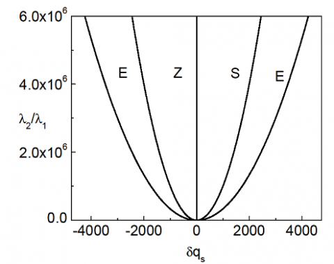
Following the subsection 4.1.1, we get domain of the zigzag instability of the form $S(+)=-{{\lambda }_{1}}q_{y}^{2}(\delta k+\frac{q_{y}^{2}}{4{{q}_{sc}}})>0$. In Figure 6, we have shown that Eckhaus instability and Zigzag instability regions.
Figure 6. Regions of Eckhuas(E), Zigzag(Z) instabilities and Stable region (S) are plotted for $Q=1000, Ta=1000, {{\sigma }_{1}}=1.5, {{\sigma }_{2}}=0.5.$
4.2 Heat transport by convection
The almost value of steady amplitude A is denoted by $|{{A}_{max}}|$ which defined as:
$|{{A}_{max}}|={{\left( \frac{{{\epsilon }^{2}}{{\lambda }_{2}}}{{{\lambda }_{3}}} \right)}^{\frac{1}{2}}},$ (46)
which is obtained from Eq. (32) with $\tanh (X/{{\Lambda }_{1}})=1$. To calculate Nusselt number $Nu$, we use $|{{A}_{max}}|$. We study the heat transfer by calculating Nusselt number $Nu$.$Nu=\frac{Hd}{\kappa \Delta T}$, where H is heat transfer per unit area which is defined as:
$H=-{{\left\langle \frac{\partial {{T}_{total}}}{\partial {z}'} \right\rangle }_{{z}'=0}}.$ (47)
In Eq. (47), angular brackets correspond to a horizontal average. We calculate the Nusselt number in terms of amplitude A in the form of:
$Nu=1+\frac{{{\epsilon }^{2}}}{\delta _{sc}^{2}}|{{A}_{max}}{{|}^{2}}.$ (48)
From Eq. (48), we obtain convection for $R>{{R}_{sc}}$ and conduction for $R\le {{R}_{sc}}$. Amplitude equation is valid for ${{\lambda }_{3}}>0$ and it is possible for $R>{{R}_{sc}}$, Thus we obtain,
1). convection for $Nu>1$ and
2). conduction for $Nu\le 1$ (Figure 7).
Figure 7. (a) is plotted for $Ta{{=10}^{3}}$ and (b) is plotted for $Ta{{=10}^{8}}$ for the fixed values of $Q=100, {{\sigma }_{1}}=0.6, {{\sigma }_{2}}=1.8$
Now consider the region near the onset of oscillatory convection. Here y-axis is taken as the axis of cylindrical rolls, so that y-dependence vanishes from Eq. $Lw=N$. The z-dependence contained entirely in $sine$ and $cosine$ functions. We introduce $\epsilon $ as:
${{\epsilon }^{2}}=\frac{{{R}_{o}}-{{R}_{oc}}}{{{R}_{oc}}}\ll 1.$ (49)
We assume that the solution of the equation $Lw=0$, which satisfies boundary conditions is of the form.
${{w}_{0}}=\left[ \begin{align} & {{A}_{1L}}{{e}^{i({{l}_{oc}}x+{{m}_{oc}}y+{{\omega }_{oc}}t)}} \\ & +{{A}_{1R}}{{e}^{i({{l}_{oc}}x+{{m}_{oc}}y-{{\omega }_{oc}}t)}}+c.c. \\\end{align} \right]\sin \pi z,$
Here ${{A}_{1L}}$ and ${{A}_{1R}}$ denotes the amplitude of left and right travelling waves of the roll, which depends on slow variables.
$X=\epsilon x,\quad Y={{\epsilon }^{\frac{1}{2}}}y,\quad \tau =\epsilon t,\quad T={{\epsilon }^{2}}t,$ (50)
and assume that ${{A}_{1L}}={{A}_{1L}}(X,\tau ,T)$, ${{A}_{1R}}={{A}_{1R}}(X,\tau ,T)$. We express the differential operators in the form of:
$\begin{align} & \frac{\partial }{\partial x}\to \frac{\partial }{\partial x}+\epsilon \frac{\partial }{\partial X},\quad \frac{\partial }{\partial y}\to \frac{\partial }{\partial y}+{{\epsilon }^{\frac{1}{2}}}\frac{\partial }{\partial Y},\quad \\ & \frac{\partial }{\partial t}\to \frac{\partial }{\partial t}+\epsilon \frac{\partial }{\partial \tau }+{{\epsilon }^{2}}\frac{\partial }{\partial T}. \\\end{align}$ (51)
We assume that the solution of basic Equations as power series in $\epsilon $,
$f=\epsilon {{f}_{0}}+{{\epsilon }^{2}}{{f}_{1}}+{{\epsilon }^{3}}{{f}_{2}}+\cdots ,$ (52)
where, $f=f(u,v,w,\theta ,{{H}_{x}},{{H}_{y}},{{H}_{z}})$ and the first approximation is given by eigenvector of the linearized problem:
$\begin{align} & {{u}_{0}}=\frac{i\pi }{{{l}_{oc}}}[{{A}_{1L}}{{e}^{i({{l}_{oc}}x+{{m}_{oc}}y+{{\omega }_{oc}}t)}} \\ & +{{A}_{1R}}{{e}^{i({{l}_{oc}}x+{{m}_{oc}}y-{{\omega }_{oc}}t)}}-c.c.]\cos \pi z, \\\end{align}$
$\begin{align}& {{v}_{0}}=\frac{\pi T{{a}^{\frac{1}{2}}}}{i{{l}_{oc}}}[{{J}_{1}}{{A}_{1L}}{{e}^{i({{l}_{oc}}x+{{m}_{oc}}y+{{\omega }_{oc}}t)}} \\ & +{{J}_{2}}{{A}_{1R}}{{e}^{i({{l}_{oc}}x+{{m}_{oc}}y-{{\omega }_{oc}}t)}}-c.c.]\cos \pi z, \\\end{align}$
${{w}_{0}}=\left[ \begin{align} & {{A}_{1L}}{{e}^{i({{l}_{oc}}x+{{m}_{oc}}y+{{\omega }_{oc}}t)}} \\& +{{A}_{1R}}{{e}^{i({{l}_{oc}}x+{{m}_{oc}}y-{{\omega }_{oc}}t)}}+c.c. \\\end{align} \right]\sin \pi z,$
$\begin{align} & {{\theta }_{0}}=[\frac{1}{\delta _{oc}^{2}+i{{\omega }_{oc}}}{{A}_{1L}}{{e}^{i({{l}_{oc}}x+{{m}_{oc}}y+{{\omega }_{oc}}t)}} \\ & +\frac{1}{\delta _{oc}^{2}-i{{\omega }_{oc}}}{{A}_{1R}}{{e}^{i({{l}_{oc}}x+{{m}_{oc}}y-{{\omega }_{oc}}t)}}+c.c.]\sin \pi z, \\\end{align}$
$\begin{align} & {{H}_{{{x}_{0}}}}=\frac{{{\pi }^{2}}}{i{{l}_{oc}}}[{{J}_{3}}{{A}_{1L}}{{e}^{i({{l}_{oc}}x+{{m}_{oc}}y+{{\omega }_{oc}}t)}} \\ & +{{J}_{4}}{{A}_{1R}}{{e}^{i({{l}_{oc}}x+{{m}_{oc}}y-{{\omega }_{oc}}t)}}-c.c.]\sin \pi z, \\\end{align}$ (53)
$\begin{align} & {{H}_{{{y}_{0}}}}=\frac{i{{\pi }^{2}}T{{a}^{\frac{1}{2}}}}{{{l}_{oc}}}[{{J}_{5}}{{A}_{1L}}{{e}^{i({{l}_{oc}}x+{{m}_{oc}}y+{{\omega }_{oc}}t)}} \\ & +{{J}_{6}}{{A}_{1R}}{{e}^{i({{l}_{oc}}x+{{m}_{oc}}y-{{\omega }_{oc}}t)}}-c.c.]\sin \pi z, \\\end{align}$
$\begin{align} & {{H}_{{{z}_{0}}}}=\pi [{{J}_{3}}{{A}_{1L}}{{e}^{i({{l}_{oc}}x+{{m}_{oc}}y+{{\omega }_{oc}}t)}} \\& +{{J}_{4}}{{A}_{1R}}{{e}^{i({{l}_{oc}}x+{{m}_{oc}}y+{{\omega }_{oc}}t)}}-c.c.]\cos \pi z. \\\end{align}$
here $\begin{align} & q_{oc}^{2}=l_{oc}^{2}+m_{oc}^{2}, \delta _{oc}^{2}=q_{oc}^{2}+{{\pi }^{2}}, {{J}_{5}}={{J}_{1}}{{J}_{3}}, {{J}_{6}}={{J}_{2}}{{J}_{4}}, \\ & {{J}_{1}}=\frac{\left( \delta _{oc}^{2}+\frac{1}{{{\sigma }_{1}}}i{{\omega }_{oc}} \right){{\left( \delta _{oc}^{2}+\frac{{{\sigma }_{2}}}{{{\sigma }_{1}}}i{{\omega }_{oc}} \right)}^{2}}}{{{\left( \delta _{oc}^{2}+\frac{1}{{{\sigma }_{1}}}i{{\omega }_{oc}} \right)}^{2}}{{\left( \delta _{oc}^{2}+\frac{{{\sigma }_{2}}}{{{\sigma }_{1}}}i{{\omega }_{oc}} \right)}^{2}}+{{Q}^{2}}{{\pi }^{2}}}, \\ & {{J}_{2}}=\frac{\left( \delta _{oc}^{2}-\frac{1}{{{\sigma }_{1}}}i{{\omega }_{oc}} \right){{\left( \delta _{oc}^{2}-\frac{{{\sigma }_{2}}}{{{\sigma }_{1}}}i{{\omega }_{oc}} \right)}^{2}}}{{{\left( \delta _{oc}^{2}-\frac{1}{{{\sigma }_{1}}}i{{\omega }_{oc}} \right)}^{2}}{{\left( \delta _{oc}^{2}-\frac{{{\sigma }_{2}}}{{{\sigma }_{1}}}i{{\omega }_{oc}} \right)}^{2}}+{{Q}^{2}}{{\pi }^{2}}}, \\ & {{J}_{3}}=\frac{1}{\delta _{oc}^{2}+\frac{{{\sigma }_{2}}}{{{\sigma }_{1}}}i{{\omega }_{oc}}}, {{J}_{4}}=\frac{1}{\delta _{oc}^{2}-\frac{{{\sigma }_{2}}}{{{\sigma }_{1}}}i{{\omega }_{oc}}} \\\end{align}$ and c.c stands for complex conjugate. By employing the definitions of Eq. (47) and Eq. (48) in to Eq. (6) and equating the coefficients of $\epsilon $, ${{\epsilon }^{2}}$, ${{\epsilon }^{3}}$ to zero, we get:
${{L}_{0}}{{w}_{0}}=0,$
${{L}_{1}}{{w}_{0}}+{{L}_{0}}{{w}_{1}}={{N}_{0}},$ (54)
${{L}_{2}}{{w}_{0}}+{{L}_{1}}{{w}_{1}}+{{L}_{0}}{{w}_{2}}={{N}_{1}},$
From the linear equation ${{L}_{0}}{{w}_{0}}=0$, we obtain the critical Rayleigh number. At $O({{\epsilon }^{2}})$, ${{N}_{0}}=0$ and ${{L}_{1}}{{w}_{0}}=0$ gives $\frac{\partial {{A}_{1L}}}{\partial \tau }-{{\nu }_{g}}\frac{\partial {{A}_{1L}}}{\partial X}=0$ and $\frac{\partial {{A}_{1L}}}{\partial \tau }+{{\nu }_{g}}\frac{\partial {{A}_{1L}}}{\partial X}=0$. Where ${{\nu }_{g}}=(\frac{\partial \omega }{\partial q}{{)}_{q={{q}_{sc}}}}$ is the group velocity and is real. Hence we get ${{u}_{1}}=0$. Similarly, the remaining first order solutions are:
${{u}_{1}}=0,$
$\begin{align} & {{v}_{1}}=\frac{\pi T{{a}^{1/2}}}{i{{l}_{sc}}{{\sigma }_{1}}}\{\frac{{{J}_{1}}}{4{{q}^{2}}+\frac{2i{{\omega }_{oc}}}{{{\sigma }_{1}}}}A_{1L}^{2}{{e}^{2i({{l}_{oc}}x+{{m}_{oc}}y+{{\omega }_{oc}}t)}} \\ & +\frac{{{J}_{2}}}{4q_{oc}^{2}-\frac{2i{{\omega }_{oc}}}{{{\sigma }_{1}}}}A_{1R}^{2}{{e}^{2i({{l}_{oc}}x+{{m}_{oc}}y-{{\omega }_{oc}}t)}} \\ & +\frac{{{J}_{1}}+{{J}_{2}}}{4q_{oc}^{2}}{{A}_{1L}}{{A}_{1R}}{{e}^{2i({{l}_{oc}}x+{{m}_{oc}}y)}}+c.c.\}, \\\end{align}$
${{w}_{1}}=0,$
$\begin{align} & {{\theta }_{1}}=\pi \{\frac{\delta _{oc}^{2}\left[ |{{A}_{1L}}{{|}^{2}}+|{{A}_{1R}}{{|}^{2}} \right]}{\delta _{oc}^{4}+\omega _{oc}^{2}} \\ & +\frac{{{A}_{1L}}A_{1R}^{*}}{\left( \delta _{oc}^{2}+i{{\omega }_{oc}} \right)\left( 2{{\pi }^{2}}+i{{\omega }_{oc}} \right)}{{e}^{2i{{\omega }_{oc}}t}}+c.c\}\sin 2\pi z, \\\end{align}$
$\begin{align} & {{H}_{{{x}_{1}}}}=\frac{\pi {{\omega }_{oc}}}{{{l}_{oc}}}\frac{\sigma _{2}^{2}}{\sigma _{1}^{2}}\frac{1}{\delta _{oc}^{4}+\omega _{oc}^{2}\frac{\sigma _{2}^{2}}{\sigma _{1}^{2}}} \\ & \left[ |{{A}_{1L}}{{|}^{2}}+|{{A}_{1R}}{{|}^{2}} \right]\sin 2\pi z, \\\end{align}$ (55)
${{H}_{{{y}_{1}}}}=0,$
$\begin{align} & {{H}_{{{z}_{1}}}}=2{{\pi }^{2}}\frac{{{\sigma }_{2}}}{{{\sigma }_{1}}}\{\frac{{{J}_{3}}}{4q_{oc}^{2}+2i{{\omega }_{oc}}}A_{1L}^{2}{{e}^{2i({{l}_{oc}}x+{{m}_{oc}}y+{{\omega }_{oc}}t)}} \\ & +\frac{2\delta _{oc}^{2}}{4{{q}^{2}}\left( \delta _{oc}^{4}+\omega _{oc}^{2}\frac{\sigma _{2}^{2}}{\sigma _{1}^{2}} \right)}{{A}_{1L}}{{A}_{1R}}{{e}^{2i({{l}_{oc}}x+{{m}_{oc}}y)}} \\\end{align}$
$+\frac{{{J}_{4}}}{4q_{oc}^{2}-2i{{\omega }_{oc}}}A_{1R}^{2}{{e}^{2i({{l}_{oc}}x+{{m}_{oc}}y-{{\omega }_{oc}}t)}}+c.c.\}.$
Equating the coefficients of $\sin \pi z$ in ${{N}_{1}}-{{L}_{2}}{{w}_{0}}$ are equal to zero. We obtain:
${{\Lambda }_{0}}\frac{\partial {{A}_{1L}}}{\partial T}+{{\Lambda }_{1}}\left( \frac{\partial }{\partial \tau }-{{v}_{g}}\frac{\partial }{\partial X} \right){{A}_{2L}}-{{\Lambda }_{2}}\frac{{{\partial }^{2}}{{A}_{1L}}}{\partial {{X}^{2}}}$$-{{\Lambda }_{3}}{{A}_{1L}}+{{\Lambda }_{4}}|{{A}_{1L}}{{|}^{2}}{{A}_{1L}}+{{\Lambda }_{5}}|{{A}_{1R}}{{|}^{2}}{{A}_{1L}}=0,$ (56)
${{\Lambda }_{0}}\frac{\partial {{A}_{1R}}}{\partial T}+{{\Lambda }_{1}}\left( \frac{\partial }{\partial \tau }-{{v}_{g}}\frac{\partial }{\partial X} \right){{A}_{2R}}-{{\Lambda }_{2}}\frac{{{\partial }^{2}}{{A}_{1R}}}{\partial {{X}^{2}}}$$-{{\Lambda }_{3}}{{A}_{1R}}+{{\Lambda }_{4}}|{{A}_{1R}}{{|}^{2}}{{A}_{1R}}+{{\Lambda }_{5}}|{{A}_{1L}}{{|}^{2}}{{A}_{1R}}=0.$ (57)
$\begin{align}& {{\Lambda }_{0}}=\delta _{oc}^{2}\left( Q{{\pi }^{2}}+{{e}_{2}}{{e}_{3}} \right)\left[ Q{{\pi }^{2}}+2\frac{{{\sigma }_{2}}}{{{\sigma }_{1}}}{{e}_{1}}{{e}_{2}}+{{e}_{3}}\left( \frac{2{{e}_{1}}}{{{\sigma }_{1}}} \right) \right] \\ & -{{R}_{oc}}q_{oc}^{2}[\frac{e_{3}^{2}}{{{\sigma }_{1}}}+\frac{{{\sigma }_{2}}}{{{\sigma }_{1}}} (Q{{\pi }^{2}}+2{{e}_{2}}{{e}_{3}})] \\ & +Ta{{\pi }^{2}}{{e}_{3}}\left( 2{{e}_{1}}\frac{{{\sigma }_{2}}}{{{\sigma }_{1}}}+{{e}_{3}} \right), \\\end{align}$$\begin{align} & {{\Lambda }_{1}}=\frac{\delta _{oc}^{2}}{\sigma _{1}^{2}}{{e}_{1}}e_{3}^{2}+\frac{2}{{{e}_{1}}}\delta _{oc}^{2}{{e}_{3}}\left( Q{{\pi }^{2}}+{{e}_{2}}{{e}_{3}} \right) \\ & +Ta{{\pi }^{2}}\frac{{{\sigma }_{2}}}{{{\sigma }_{1}}}\left( {{e}_{1}}\frac{{{\sigma }_{2}}}{{{\sigma }_{1}}}+2{{e}_{3}} \right) \\ & +\frac{2}{{{e}_{1}}}\frac{{{\sigma }_{2}}}{{{\sigma }_{1}}}\left( {{e}_{1}}\delta _{oc}^{2}\left( Q{{\pi }^{2}}+2{{e}_{2}}{{e}_{3}} \right)+{{R}_{oc}}q_{oc}^{2}{{e}_{3}} \right) \\\end{align}$
$\begin{align}& +\frac{{{\sigma }_{2}}}{{{\sigma }_{1}}}{{e}_{2}}[{{R}_{oc}}q_{oc}^{2}\frac{{{\sigma }_{2}}}{{{\sigma }_{1}}} \\ & +\delta _{oc}^{2}({{e}_{1}}\left( {{e}_{1}}\frac{{{\sigma }_{2}}}{{{\sigma }_{1}}}+2{{e}_{3}} \right)+2Q{{\pi }^{2}})], \\ & {{\Lambda }_{2}}=Q{{\pi }^{2}}[{{R}_{oc}}-Q{{\pi }^{2}} \\ & -2({{e}_{1}}{{e}_{2}}+{{e}_{2}}{{e}_{3}}+{{e}_{1}}{{e}_{3}}+\delta _{oc}^{2}({{e}_{1}}+{{e}_{2}}+{{e}_{3}}))] \\& +{{R}_{oc}}[{{e}_{2}}(q_{oc}^{2}+2{{e}_{3}})+{{e}_{3}}(2q_{oc}^{2}+{{e}_{3}})] \\ & -2Ta{{\pi }^{2}}({{e}_{1}}{{e}_{2}}+{{e}_{3}})-\delta _{oc}^{2}[2{{e}_{3}}{{e}_{2}}({{e}_{2}}+{{e}_{3}}) \\ & +{{e}_{1}}(e_{1}^{2}+e_{3}^{2})+4{{e}_{1}}{{e}_{2}}{{e}_{3}}-{{e}_{3}}{{e}_{2}}({{e}_{3}}{{e}_{2}}+2{{e}_{1}}({{e}_{2}}+e_{3}^{3})), \\ & {{\Lambda }_{3}}=R_{oc}^{2}q_{oc}^{2}{{e}_{2}}\left( Q{{\pi }^{2}}+{{e}_{2}}{{e}_{3}} \right), \\\end{align}$
$\begin{align} & {{\Lambda }_{4}}=\left( Q{{\pi }^{2}}+{{e}_{2}}{{e}_{3}} \right)\{Q{{\pi }^{2}}\frac{\sigma _{2}^{2}}{\sigma _{1}^{2}}\frac{{{e}_{1}}}{{{e}_{4}}}[\frac{i{{\omega }_{oc}}{{\sigma }_{2}}}{{{\sigma }_{1}}} \\ & \left( (3{{\pi }^{2}}-l_{oc}^{2})-\frac{\delta _{oc}^{2}{{\pi }^{2}}}{2{{e}_{3}}{{l}_{oc}}} \right)-\frac{{{\pi }^{2}}{{e}_{3}}}{i{{l}_{oc}}}\frac{{{\pi }^{2}}-2l_{oc}^{2}}{2q_{oc}^{2}+i{{\omega }_{oc}}} \\& +\frac{\delta _{oc}^{2}{{\pi }^{2}}{{\omega }_{oc}}}{2{{l}_{oc}}}] \\\end{align}$
$\begin{align} & +\frac{\sigma _{2}^{2}}{\sigma _{1}^{2}}\frac{Q\delta _{oc}^{2}{{\pi }^{4}}}{2q_{oc}^{2}+i{{\omega }_{oc}}}-\frac{{{R}_{oc}}{{e}_{3}}{{\pi }^{2}}q_{oc}^{2}\delta _{oc}^{2}}{\delta _{oc}^{4}+\omega _{oc}^{2}}\}+Ta{{e}_{2}}{{e}_{3}} \\ & [\frac{{{\sigma }_{2}}}{{{\sigma }_{1}}}\frac{{{e}_{5}}{{\pi }^{4}}}{4q_{oc}^{2}+2i{{\omega }_{oc}}}-\frac{{{\omega }_{oc}}}{{{e}_{4}}}\frac{\sigma _{2}^{2}}{\sigma _{1}^{2}}(i{{\pi }^{4}}+{{J}_{1}}\frac{{{\omega }_{oc}}}{2}) \\ & -\frac{1}{\sigma _{1}^{2}}\frac{{{J}_{1}}{{\pi }^{3}}}{2q_{oc}^{2}+i{{\omega }_{oc}}}] \\ & {{\Lambda }_{5}}=\left( Q{{\pi }^{2}}+{{e}_{2}}{{e}_{3}} \right)\{Q{{\pi }^{2}}\frac{\sigma _{2}^{2}}{\sigma _{1}^{2}}\frac{{{e}_{1}}}{{{e}_{4}}}[\frac{{{\omega }_{oc}}{{\sigma }_{2}}}{{{\sigma }_{1}}} \\ & \left( i(3{{\pi }^{2}}+l_{oc}^{2})-\frac{\delta _{oc}^{2}{{\pi }^{2}}}{2{{e}_{3}}{{l}_{oc}}} \right)-\pi \frac{\delta _{oc}^{2}}{q_{oc}^{2}}(2{{\pi }^{2}}-4l_{oc}^{2}-\pi \delta _{oc}^{2})] \\ & -\frac{{{R}_{oc}}{{e}_{3}}{{\pi }^{2}}q_{oc}^{2}\delta _{oc}^{2}}{\delta _{oc}^{4}+\omega _{oc}^{2}}\}+Ta{{e}_{2}}{{e}_{3}}\{\frac{{{\pi }^{3}}}{2q_{oc}^{2}}\frac{{{J}_{1}}+{{J}_{2}}}{{{\sigma }_{1}}} \\\end{align}$ (58)
$\begin{align} & \left( 1+Q{{\pi }^{2}}{{J}_{3}}\frac{{{\sigma }_{2}}}{{{\sigma }_{1}}} \right)+\frac{{{\pi }^{4}}}{{{e}_{4}}}\frac{{{\sigma }_{2}}}{{{\sigma }_{1}}}[\frac{i{{\omega }_{oc}}}{2}\frac{{{\sigma }_{2}}}{{{\sigma }_{1}}}\left( {{J}_{5}}-Q\frac{{{\sigma }_{2}}}{{{\sigma }_{1}}} \right) \\ & +\frac{\delta _{oc}^{2}}{q_{oc}^{2}}\left( Q{{\pi }^{2}}\frac{{{\sigma }_{2}}}{{{\sigma }_{1}}}-\frac{J_{6}^{*}}{2} \right)]\}. \\\end{align}$
where, ${{\Lambda }_{0}}$, ${{\Lambda }_{1}}$, ${{\Lambda }_{2}}$, ${{\Lambda }_{3}}$, ${{\Lambda }_{4}}$ and ${{\Lambda }_{5}}$ are the complex coefficients in physical components ${{q}_{oc}}$, $Q$ and $Ta$. Here, $\begin{align} & {{e}_{1}}=\delta _{oc}^{2}+i{{\omega }_{oc}}, {{e}_{2}}=\delta _{oc}^{2}+i{{\omega }_{oc}}\frac{1}{{{\sigma }_{1}}}, \\ & {{e}_{3}}=\delta _{oc}^{2}+i{{\omega }_{oc}}\frac{{{\sigma }_{2}}}{{{\sigma }_{1}}}, {{e}_{4}}=\delta _{oc}^{4}+\omega _{oc}^{2}\frac{\sigma _{2}^{2}}{\sigma _{1}^{2}}, \\\end{align}$ ${{e}_{5}}=2Q{{\pi }^{2}}J_{1}^{*}{{J}_{3}}\frac{{{\sigma }_{2}}}{{{\sigma }_{1}}}-Q\pi {{J}_{1}}(1+J_{3}^{*})\frac{1}{{{\sigma }_{1}}}-2i{{\pi }^{2}}J_{5}^{*}\frac{1}{{{e}_{3}}}.$
Here${{A}_{2L}}=(\frac{\partial }{\partial \tau }+{{\nu }_{g}}\frac{\partial }{\partial X}){{A}_{1L}}$ and ${{A}_{2R}}=(\frac{\partial }{\partial \tau }-{{\nu }_{g}}\frac{\partial }{\partial X}){{A}_{1R}}$. ${{A}_{1L}}$, ${{A}_{1R}}$ and ${{A}_{2L}}$, ${{A}_{2R}}$ are of orders $\epsilon $ and ${{\epsilon }^{2}}$ respectively. From the Eqns. $\frac{\partial {{A}_{1L}}}{\partial \tau }-{{\nu }_{g}}\frac{\partial {{A}_{1L}}}{\partial X}=0$ and$\frac{\partial {{A}_{1L}}}{\partial \tau }+{{\nu }_{g}}\frac{\partial {{A}_{1L}}}{\partial X}=0$ we obtain ${{A}_{1L}}({\xi }',T)$ and ${{A}_{1R}}({\eta }',T)$. Where ${\xi }'={{\nu }_{g}}\tau +X$ ${\eta }'={{\nu }_{g}}\tau -X$. Eqns. (52) and (53) can be written as:
$\begin{align} & 2{{v}_{g}}{{\Lambda }_{1}}\frac{\partial {{A}_{2L}}}{\partial {\eta }'}=-{{\Lambda }_{0}}\frac{\partial {{A}_{1L}}}{\partial T}+{{\Lambda }_{2}}\frac{\partial {{A}_{1L}}}{\partial {{X}^{2}}}+{{\Lambda }_{3}}{{A}_{1L}} \\ & -\left( {{\Lambda }_{4}}|{{A}_{1L}}{{|}^{2}}+{{\Lambda }_{5}}|{{A}_{1R}}{{|}^{2}} \right){{A}_{1L}}, \\\end{align}$ (59)
$\begin{align} & 2{{v}_{g}}{{\Lambda }_{1}}\frac{\partial {{A}_{2R}}}{\partial {\eta }'}=-{{\Lambda }_{0}}\frac{\partial {{A}_{1R}}}{\partial T}+{{\Lambda }_{2}}\frac{\partial {{A}_{1R}}}{\partial {{X}^{2}}}+{{\lambda }_{3}}{{A}_{1R}} \\& -\left( {{\Lambda }_{4}}|{{A}_{1R}}{{|}^{2}}+{{\Lambda }_{5}}|{{A}_{1L}}{{|}^{2}} \right){{A}_{1R}}. \\\end{align}$ (60)
Let ${\xi }'\epsilon [0,{{l}_{1}}]$, ${\eta }'\epsilon [0,{{l}_{2}}]$ where ${{l}_{1}}$ is the period of ${{A}_{1L}}$ and ${{l}_{2}}$ is the period of ${{A}_{1R}}$ . Eq. (48) remains asymptotic for times $t=O\left( {{\epsilon }^{-2}} \right)$ only if an appropriate solvability condition holds. This condition derived by integrating Eq. (59) over ${\eta }'$ and Eq. (60) over ${\xi }'$, we obtain,
$\begin{align} & {{\Lambda }_{0}}\frac{\partial {{A}_{1L}}}{\partial T}={{\Lambda }_{2}}\frac{\partial {{A}_{1L}}}{\partial {{X}^{2}}}+{{\lambda }_{3}}{{A}_{1L}} \\ & -\left( {{\Lambda }_{4}}|{{A}_{1L}}{{|}^{2}}+{{\Lambda }_{5}}|{{A}_{1R}}{{|}^{2}} \right){{A}_{1L}}, \\\end{align}$ (61)
$\begin{align} & {{\Lambda }_{0}}\frac{\partial {{A}_{1R}}}{\partial T}={{\Lambda }_{2}}\frac{\partial {{A}_{1R}}}{\partial {{X}^{2}}}+{{\lambda }_{3}}{{A}_{1R}} \\& -\left( {{\Lambda }_{4}}|{{A}_{1R}}{{|}^{2}}+{{\Lambda }_{5}}|{{A}_{1L}}{{|}^{2}} \right){{A}_{1R}}. \\\end{align}$ (62)
The Eqns. (61) and (62) are for the amplitudes of left and right moving waves respectively. These equations are known as one-dimensional coupled Landau-Ginzburg equations with original slow spatial coordinate and time.
5.1 Travelling wave and standing wave convection
On dropping slow variable X from Eqns. (61) and (62), we obtain a system of first order ODE’s.
$\begin{align} & \frac{\text{d}{{A}_{1L}}}{\text{d}T}=\frac{{{\Lambda }_{3}}}{{{\Lambda }_{0}}}{{A}_{1L}}-\frac{{{\Lambda }_{4}}}{{{\Lambda }_{0}}}{{A}_{1L}}|{{A}_{1L}}{{|}^{2}} \\ & -\frac{{{\Lambda }_{5}}}{{{\Lambda }_{0}}}{{A}_{1L}}|{{A}_{1R}}{{|}^{2}}, \\\end{align}$ (63)
$\frac{\text{d}{{A}_{1R}}}{\text{d}T}=\frac{{{\Lambda }_{3}}}{{{\Lambda }_{0}}}{{A}_{1R}}-\frac{{{\Lambda }_{4}}}{{{\Lambda }_{0}}}{{A}_{1R}}|{{A}_{1R}}{{|}^{2}}-\frac{{{\Lambda }_{5}}}{{{\Lambda }_{0}}}{{A}_{1R}}|{{A}_{1L}}{{|}^{2}}.$ (64)
Put $\beta =\frac{{{\Lambda }_{3}}}{{{\Lambda }_{0}}},\quad \gamma =-\frac{{{\Lambda }_{4}}}{{{\Lambda }_{0}}}\quad and\quad \delta =-\frac{{{\Lambda }_{5}}}{{{\Lambda }_{0}}}.$
Then Eqns. (63) and (64) take the following form:
$\frac{\text{d}{{A}_{1L}}}{\text{d}T}={\beta }'{{A}_{1L}}+{\gamma }'{{A}_{1L}}|{{A}_{1L}}{{|}^{2}}+{\delta }'{{A}_{1L}}|{{A}_{1R}}{{|}^{2}},$ (65)
$\frac{\text{d}{{A}_{1R}}}{\text{d}T}={\beta }'{{A}_{1R}}+{\gamma }'{{A}_{1R}}|{{A}_{1R}}{{|}^{2}}+{\delta }'{{A}_{1R}}|{{A}_{1L}}{{|}^{2}}.$ (66)
Consider ${{A}_{1L}}={{a}_{L}}{{e}^{i{{\phi }_{L}}}}$ and ${{A}_{1R}}={{a}_{L}}{{e}^{i{{\phi }_{R}}}}$, where ${{a}_{L}}=|{{A}_{1L}}|$, ${{\phi }_{L}}=arg({{A}_{1L}})=\mathop{\tan }^{-1}\left( Im({{A}_{1L}})/Re({{A}_{1L}}) \right)$ and ${{a}_{R}}=|{{A}_{1R}}|$, ${{\phi }_{R}}=arg({{A}_{1R}})=\mathop{\tan }^{-1}(\frac{Im({{A}_{1R}})}{Re({{A}_{1R}})})$, here ${{a}_{L}}$, ${{a}_{R}}$, ${{\phi }_{L}}$ and ${{\phi }_{R}}$ are functions of time $T$. Clearly ${{a}_{L}}$ and ${{a}_{R}}$ are positive functions. Putting ${{A}_{1L}}={{a}_{L}}{{e}^{i{{\phi }_{L}}}}$, ${{A}_{1R}}={{a}_{L}}{{e}^{i{{\phi }_{R}}}}$ and ${\beta }'={{\beta }_{1}}+i{{\beta }_{2}}$, ${\gamma }'={{\gamma }_{1}}+i{{\gamma }_{2}}$, ${\delta }'={{\delta }_{1}}+i{{\delta }_{2}}$ into Eqns. (65) and (66) we get,
$\frac{\text{d}{{a}_{L}}}{\text{d}T}={{\beta }_{1}}{{a}_{L}}+{{\gamma }_{1}}{{a}_{L}}|{{a}_{L}}{{|}^{2}}+{{\delta }_{1}}{{a}_{L}}|{{a}_{R}}{{|}^{2}},$ (67)
$\frac{\text{d}{{\phi }_{L}}}{\text{d}T}={{\beta }_{2}}+{{\gamma }_{2}}|{{a}_{L}}{{|}^{2}}+{{\delta }_{2}}|{{a}_{R}}{{|}^{2}},$ (68)
$\frac{\text{d}{{a}_{R}}}{\text{d}T}={{\beta }_{1}}{{a}_{R}}+{{\gamma }_{1}}{{a}_{R}}|{{a}_{R}}{{|}^{2}}+{{\delta }_{1}}{{a}_{R}}|{{a}_{L}}{{|}^{2}},$ (69)
$\frac{\text{d}{{\phi }_{R}}}{\text{d}T}={{\beta }_{2}}+{{\gamma }_{2}}|{{a}_{R}}{{|}^{2}}+{{\delta }_{2}}|{{a}_{L}}{{|}^{2}}.$ (70)
Since the Eqns. (67) and (69) does not contain phase term, so that we consider these two equations for the further discussions. Let us consider the Eqns. (67) and (69) as:
$\frac{\text{d}{{a}_{L}}}{\text{d}T}={{\beta }_{1}}{{a}_{L}}+{{\gamma }_{1}}a_{L}^{3}+{{\delta }_{1}}a_{R}^{2},$ (71)
$\frac{\text{d}{{a}_{R}}}{\text{d}T}={{\beta }_{1}}{{a}_{R}}+{{\gamma }_{1}}a_{R}^{3}+{{\delta }_{1}}a_{L}^{2}.$ (72)
Since ${{a}_{L}}$ and ${{a}_{R}}$ are positive functions. Put,
$\frac{\text{d}{{a}_{L}}}{\text{d}T}={{F}_{1}}({{a}_{L}},{{a}_{R}}),\quad \frac{\text{d}{{a}_{R}}}{\text{d}T}={{F}_{2}}({{a}_{L}},{{a}_{R}}).$ (73)
Let us discuss the stability of equilibrium points of above Eq. (73). We obtain four equilibrium points, i.e.,
1). $({{a}_{L}},{{a}_{R}})=(0,0),$
2). $({{a}_{L}},{{a}_{R}})=({{a}_{L}},0),$
3). $({{a}_{L}},{{a}_{R}})=(0,{{a}_{R}}),$
4). for ${{a}_{L}}\ne 0$ and ${{a}_{R}}\ne 0$ we obtain $({{a}_{L}},{{a}_{R}})=\left( -\frac{{{\beta }_{1}}}{{{\gamma }_{1}}+{{\delta }_{1}}},-\frac{{{\beta }_{1}}}{{{\gamma }_{1}}+{{\delta }_{1}}} \right)$.
From these points we can say the conditions for Travelling Waves and Standing Waves. The conditions for TW and SW are ${{A}_{L}}={{A}_{R}}$ and ${{A}_{L}}=0$ or ${{A}_{R}}=0$.
Travelling Waves exist if $|{{A}_{L}}{{|}^{2}}=-\frac{{{\beta }_{1}}}{{{\gamma }_{1}}}>0$ and they are supercritical if ${{\gamma }_{1}}<0$. Standing Waves exist if $|{{A}_{L}}{{|}^{2}}=|{{A}_{L}}{{|}^{2}}=-\frac{{{\beta }_{1}}}{{{\gamma }_{1}}+{{\delta }_{1}}}>0$ and supercritical if ${{\gamma }_{1}}+{{\delta }_{1}}<0$.
Also, TW are stable if ${{\beta }_{1}}>0,{{\gamma }_{1}}<0$ and ${{\delta }_{1}}<{{\gamma }_{1}}<0$.
SW are stable if ${{\beta }_{1}}>0,{{\gamma }_{1}}<0$ and
(i) if ${{\delta }_{1}}>0$, then $-{{\gamma }_{1}}>{{\delta }_{1}}>0$,
(ii) if ${{\delta }_{1}}<0$, then $-{{\gamma }_{1}}>-{{\delta }_{1}}>0$.
Figure 8. Stability regions of Travelling waves (TW), Standing waves (SW) and steady state (SS) are plotted for ${{\sigma }_{2}}=0.5$, (a) $Ta=1000$, (b) $Q=1000$
The nonlinear magneto convection in rotating fluid due to vertical magnetic field and vertical axis of rotation are analyzed. The problem was examined by using normal mode method by performing linear and weakly nonlinear analyses. The stationary Rayleigh number (Rs) and oscillatory Rayleigh number (Ro) versus wave numbers are described graphically. Takens-Bogdanov bifurcation point had obtained. In order to study the secondary instabilities viz. Eckhaus instability and Zigzag instability the well-known equation, Ginzburg-Landau equation has been derived.
The system of coupled nonlinear one-dimensional amplitude equations is also derived. The stability regions for both Standing waves (${{A}_{1L}}={{A}_{1R}}$) and Travelling waves (${{A}_{1L}}=0$ or ${{A}_{1R}}=0$) are identified. Travelling waves exist if $|{{A}_{1R}}{{|}^{2}}=-\frac{{{\beta }_{1}}}{{{\gamma }_{1}}}>0$ and they are supercritical if ${{\gamma }_{1}}<0$. Standing waves exist if $|{{A}_{1L}}{{|}^{2}}=|{{A}_{1R}}{{|}^{2}}=-\frac{{{\beta }_{1}}}{{{\gamma }_{1}}+{{\zeta }_{1}}}>0$ and they are supercritical if ${{\gamma }_{1}}+{{\zeta }_{1}}<0$ (Figure 8).
The work reported in this paper is supported by SERB of India (Order No. SB/EMEQ-482/2014). The authors gratefully acknowledge the support thus received.
${{k}_{1}}=-{{\delta }^{2}}s_{1}^{3}s_{2}^{4},$
$\begin{align} & {{k}_{3}}=({{\delta }^{6}}{{s}_{2}}s_{3}^{2}-3{{\delta }^{2}}{{s}_{1}}s_{2}^{2}{{s}_{4}})({{s}_{4}}-{{s}_{1}}{{\delta }^{4}})+({{s}_{2}}-1)({{\delta }^{10}}s_{3}^{3} \\ & -2{{\delta }^{6}}{{s}_{1}}{{s}_{2}}{{s}_{3}}{{s}_{4}}) \\ & +Ta{{\pi }^{2}}s_{2}^{2}\left( -{{s}_{2}}{{s}_{4}}+{{\delta }^{4}}({{s}_{1}}(1-{{s}_{2}})+{{s}_{3}}(1+{{s}_{2}})) \right), \\\end{align}$
$\begin{align} & {{k}_{4}}={{\delta }^{2}}{{s}_{4}}\left[ {{s}_{2}}{{s}_{4}}({{s}_{4}}-3{{s}_{1}}{{\delta }^{4}})+{{\delta }^{4}}{{s}_{3}}{{s}_{4}}({{s}_{2}}-1)+{{\delta }^{8}}s_{3}^{2} \right] \\ & +Ta{{\pi }^{2}}{{\delta }^{8}}{{s}_{3}}({{s}_{2}}+1)-Ta{{\pi }^{2}}{{\delta }^{4}}{{s}_{2}}({{s}_{4}}+{{s}_{1}}{{\delta }^{4}}-{{s}_{2}}{{s}_{4}}), \\\end{align}$
${{k}_{5}}={{\delta }^{6}}{{s}_{4}}(s_{4}^{2}+Ta{{\pi }^{2}}{{\delta }^{2}}),$
${{k}_{6}}={{\delta }^{4}}s_{1}^{2}s_{2}^{3}\left( {{s}_{1}}({{s}_{2}}-1)+{{s}_{3}} \right),$
$\begin{aligned}
&k_{7}=s_{2} \delta^{2}\left[\delta^{2}\left[\begin{array}{l}
s_{1}^{2} s_{2}\left(s_{3} \delta^{4}+3 s_{4}\left(1-s_{2}\right)\right) \\
+s_{1} s_{3}\left(s_{3} \delta^{4}\left(s_{2}-1\right)-2 s_{2} s_{4}\right)
\end{array}\right]\right. \\
&\left.\delta^{6} s_{3}^{3}-T a \pi^{2} s_{2}^{2}\left(s_{1}\left(s_{2}+1\right)-s_{3}\right)\right]
\end{aligned}$,
$\begin{align} & {{k}_{8}}={{\delta }^{2}}[{{\delta }^{2}}\left[ {{s}_{2}}{{s}_{3}}{{s}_{4}}({{s}_{4}}-2{{s}_{1}}{{\delta }^{4}})-{{\delta }^{4}}s_{3}^{2}{{s}_{4}}({{s}_{2}}-1)+{{\delta }^{8}}s_{3}^{3} \right] \\ & 3{{s}_{1}}{{s}_{2}}s_{4}^{2}{{\delta }^{2}}({{s}_{2}}-1) \\ & +Ta{{\pi }^{2}}{{s}_{2}}\left[ ({{s}_{2}}+1)({{s}_{2}}{{s}_{4}}-{{s}_{1}}{{\delta }^{4}})-{{\delta }^{4}}{{s}_{3}}({{s}_{2}}-1) \right]], \\\end{align}$
${{k}_{9}}={{\delta }^{4}}s_{4}^{2}({{s}_{3}}{{\delta }^{4}}+{{s}_{4}}(1-{{s}_{2}}))+Ta{{\pi }^{2}}{{\delta }^{6}}({{s}_{4}}({{s}_{2}}+1)-{{\delta }^{4}}{{s}_{3}}),$
${{k}_{10}}=s_{1}^{2}s_{2}^{4},$
${{k}_{11}}=s_{2}^{2}({{\delta }^{4}}(s_{1}^{2}+s_{3}^{2})-2{{s}_{1}}{{s}_{2}}{{s}_{4}}),$
${{k}_{12}}={{s}_{2}}{{s}_{4}}({{s}_{2}}{{s}_{4}}-2{{s}_{1}}{{\delta }^{4}})+{{\delta }^{8}}s_{3}^{2},$${{k}_{13}}=s_{4}^{2}{{\delta }^{4}}.$
where, ${{s}_{1}}=\frac{1}{{{\sigma }_{1}}}, {{s}_{2}}=\frac{{{\sigma }_{2}}}{{{\sigma }_{1}}}, {{s}_{3}}={{s}_{1}}+{{s}_{2}}, {{s}_{4}}={{\delta }^{4}}+Q{{\pi }^{2}}$ and ${{\delta }^{2}}={{\pi }^{2}}+{{q}^{2}}$.
[1] Huppert, H.E., Turner, J.S. (1981). Double-diffusive convection. Journal of Fluid Mechanics, 106: 299-329. https://doi.org/10.1017/S0022112081001614
[2] Tagare, S.G. (1997). Nonlinear stationary magnetoconvection in a rotating fluid. Journal of Plasma Physics, 58(3): 395-408. https://doi.org/10.1017/S0022377897006004
[3] Drazin, P.G., Reid, W.H. (2004). Hydrodynamic stability. Cambridge University Press.
[4] Eltayeb, I.A. (1975). Overstable hydromagnetic convection in a rotating fluid layer. Journal of Fluid Mechanics, 71(1): 161-179. https://doi.org/10.1017/S0022112075002480
[5] Jones, C.A., Roberts, P.H. (2000). The onset of magnetoconvection at large Prandtl number in a rotating layer II. Small magnetic diffusion. Geophysical & Astrophysical Fluid Dynamics, 93(3-4): 173-226. https://doi.org/10.1080/03091920008204124
[6] Roberts, P.H., Jones, C.A. (2000). The onset of magnetoconvection at large Prandtl number in a rotating layer I. Finite magnetic diffusion. Geophysical & Astrophysical Fluid Dynamics, 92(3-4): 289-325. https://doi.org/10.1080/03091920008203719
[7] Soward, A.M. (1980). Finite-amplitude thermal convection and geostrophic flow in a rotating magnetic system. Journal of Fluid Mechanics, 98(3): 449-471. https://doi.org/10.1017/S0022112080000249
[8] Tagare, S.G., Babu, A.B., Rameshwar, Y. (2008). Rayleigh–Benard convection in rotating fluids. International Journal of Heat and Mass Transfer, 51(5-6): 1168-1178. https://doi.org/10.1016/j.ijheatmasstransfer.2007.03.052
[9] Babu, A.B., Shanker, B., Tagare, S.G. (2011). Non-linear convection due to compositional and thermal buoyancy in Earth's outer core. International Journal of Non-Linear Mechanics, 46(7): 919-930. https://doi.org/10.1016/j.ijnonlinmec.2011.04.002
[10] Babu, A.B., Ravi, R., Tagare, S.G. (2014). Nonlinear thermohaline magnetoconvection in a sparsely packed porous medium. Journal of Porous Media, 17(1): 31-57. https://doi.org/10.1615/JPorMedia.v17.i1.30
[11] Ravi, R., Kanchana, C., Siddheshwar, P.G. (2017). Effects of second diffusing component and cross diffusion on primary and secondary thermoconvective instabilities in couple stress liquids. Applied Mathematics and Mechanics, 38(11): 1579-1600. http://dx.doi.org/10.1007/s10483-017-2280-9
[12] Newell, A.C., Whitehead, J.A. (1969). Finite bandwidth, finite amplitude convection. Journal of Fluid Mechanics, 38(2): 279-303. https://doi.org/10.1017/S0022112069000176
[13] Guba, P., Worster, M.G. (2010). Interactions between steady and oscillatory convection in mushy layers. Journal of Fluid Mechanics, 645: 411-434. 10.1017/S0022112009992709
[14] Matthews, P.C., Ruckllidge, A.M. (1993). Travelling and standing waves in magnetoconvection. Proceedings of the Royal Society of London. Series A: Mathematical and Physical Sciences, 441(1913): 649-658. https://doi.org/10.1098/rspa.1993.0085
[15] Knobloch, E., Silber, M. (1990). Travelling wave convection in a rotating layer. Geophysical & Astrophysical Fluid Dynamics, 51(1-4): 195-209. https://doi.org/10.1080/03091929008219856
[16] Avula, B.B., Venkata Koteswara Rao, N., Tagare, S.G. (2019). Instabilities of horizontal magnetoconvection with rotating fluid in a sparsely packed porous media. Heat Transfer-Asian Research, 48(7): 3055-3078. https://doi.org/10.1002/htj.21530
[17] Babu, A.B., Koteswararao, N.V. (2019). Nonlinear instabilities of horizontal magnetoconvection in a sparsely packed porous medium. Special Topics & Reviews in Porous Media: An International Journal, 10(5): 503-523. https://doi.org/10.1615/SpecialTopicsRevPorousMedia.2020026933