Xiaoye Sun* | Fuming Chen | Zhian Pan | Ling Bai
© 2021 IIETA. This article is published by IIETA and is licensed under the CC BY 4.0 license (http://creativecommons.org/licenses/by/4.0/).
OPEN ACCESS
At this critical junction of industrialization, China is facing an increasingly prominent imbalance between energy supply and demand. It is of great social significance to study the energy-saving of buildings that consume a huge amount of energy. For most heating systems, energy waste mainly arises from inefficient operations of boilers, low efficiency of pipe transmission, and poor quality of heat supply. This paper researches and evaluates the energy-saving reconstruction of intelligent community heating (ICH) system based on the Internet of things (IoT). Firstly, the energy-saving reconstruction of the ICH system was analyzed, and a hydraulic regime model was derived from the simplified model of the water supply and return pipe networks. Then, the system pipe network was investigated in three aspects, namely, node flow balance, pipeline pressure drop balance, and loop pressure drop balance. On this basis, the authors presented the balance equation and finalized the hydraulic regime model of the system. After that, the energy consumption of the system was evaluated before and after the reconstruction, and the energy-saving benefit was predicted. The effectiveness of the proposed method was proved through experiments.
internet of things (IoT), intelligent community heating (ICH), energy-saving reconstruction, energy-saving evaluation
At this critical junction of industrialization, China is facing an increasingly prominent imbalance between energy supply and demand. It is urgent to innovate the institutions and technologies in the energy sector. Buildings that consume a huge amount of energy boast a great potential of energy-saving [1-5]. According to Energy Conservation Design Standard for New Heating Residential Buildings (JGJ 26-1995), the centralized community heating system, which consists of a heat source like boiler room/thermal power plant, an outdoor heating pipe network, and indoor heating terminals, should reach an energy-saving rate of 20% [6-8]. However, most of the existing heating systems cannot live up to this standard. More advanced means is needed to effectively enhance the heating efficiency of heating systems [9-13].
Kobzar et al. [14] analyzed the energy efficiency of a community heating system after energy-saving reconstruction, and evaluated the energy efficiency in terms of heating quality, heating cost, and environmental benefit, according to the real-time energy consumption in the heating season. Abdelaziz et al. [15] examined the distribution features of heating buildings in regional economic development zones, developed a regional intelligent heating monitoring system based on the Internet of things (IoT), and applied the system to real-time remote monitoring of the planned heating pipe network. Hwang and Jeong [16] constructed an IoT-based college heating system, divided the network nodes in the system (e.g., decentralized heating and room temperature compensation controllers), and realized the remote monitoring based on remote control center and online interactions.
To improve the scientific level of system design data, improve the energy-saving analysis in operation and management, and create a comfortable indoor heating environment, it is necessary to integrate intelligent control technologies that can elevate the automation of heating system with building information modeling (BIM) [17-21]. Long et al. [22] developed a heat source for college heating system through intelligent frequency conversion, realized the dynamic intelligent heating control of heat source, water supply pipe network, water return pipe network, and buildings by adjusting and transforming valve layout, and introduced the BIM technology that analyzes the mean indoor thermal sensation index and computes real-time dynamic heat load, thereby achieving the data upload to operation and maintenance platform and real-time control of the center of the intelligent control system. Sun et al. [23] designed the proportional-integration-derivative (PID) control algorithm for backpropagation neural network (BPNN), and effectively controlled the real-time opening of intelligent balance valves in community heating system.
For most heating systems, energy waste mainly arises from inefficient operations of boilers, low efficiency of pipe transmission, and poor quality of heat supply. Therefore, it is of high necessity to analyze the energy consumption of the heating system, and reconstruct the system for better energy efficiency [24-28]. This paper researches and evaluates the energy-saving reconstruction of intelligent community heating (ICH) system based on IoT. Section 2 analyzes the energy-saving reconstruction of the ICH system, simplifies the water supply and return pipe networks, and constructs the hydraulic regime model of the simplified model, laying the basis for IoT-based analysis of energy-saving reconstruction. Section 3 explores the system pipe network in three aspects, namely, node flow balance, pipeline pressure drop balance, and loop pressure drop balance, and presents the balance equation and finalizes the hydraulic regime model of the system. Section 4 analyzes the energy consumption of the system before and after the reconstruction, and predicts the energy-saving benefit of the system. The effectiveness of the proposed method was proved through experiments.
In an intelligent community, the heating demand of buildings increases with the occupancy rate. The IoT-based energy-saving reconstruction of ICH system requires the verification of hydraulic regime and redesign of heating meter distribution in the current water supply and return pipe networks. This is to ensure the real-time collection and processing of heat supply data, and automate the control of heat supply and distribution, without sacrificing the heating demand and safety of community users.
2.1 Pipe network simplification
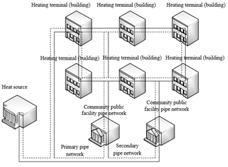
Figure 1. Simplified structure of community heating system
The water supply and return network of ICH system should be simplified under the principle of maintaining the correlations between network nodes and pipes, and minimizing the error relative to the actual system. Figure 1 provides the simplified structure of community heating system. The direction of hot water flowing in the pipeline could be simplified as the direction of an edge in the directed graph DBS of the water supply and return network, where ui is heating nodes in the graph, ri is the heating pipeline connected to heating node u, and g is the relationship between ui and ri. Then, the directed graph can be defined as:
$D_{B S}=g\left(u_{i}, r_{i}\right)$ (1)
Suppose the directed graph DBS of the simplified water supply and return network has a total of NP heating pipelines, NNO heating nodes, Q heating branches, and V heating loops. Let R and U be the set of heating pipelines, and the set of heating nodes, respectively. Then, the following can be derived from the Euler formula:
$V+M_{N O}=N_{P}+Q$ (2)
This paper describes the correlations between all the heating pipelines and heating nodes as an incidence matrix of pipeline correlations. Then, the augmented incidence matrix F of water supply and return network can be described by:
$F\left(D_{B S}\right)=\left\{f_{i j}\right\}$ (3)
The elements in matrix F can be described by a ternary function:
${{f}_{ij}}=\left\{ \begin{align} & 1\text{ }{{u}_{i}}\text{ }is\text{ }the\text{ }starting\text{ }point\text{ }of\text{ }{{r}_{i}} \\ & 0\text{ }{{u}_{i}}\text{ }is\text{ }not\text{ }correlated\text{ }with\text{ }{{r}_{i}} \\ & -1\text{ }{{u}_{i}}\text{ }is\text{ }the\text{ }ending\text{ }point\text{ }of\text{ }{{r}_{i}} \\\end{align} \right.$ (4)
In the water supply and return network, the correlations between the basic heating loop and the heating pipelines could be described by a loop incidence matrix. The number of heating loops V equals Q-NNO+1. The loop incidence matrix can be described by H(DBS)={hij}. The elements of matrix H can be described by a ternary function:
$h_{i j}=\left\{\begin{array}{cc}1 & r_{i} \text { flows in the same } \\ & \text { direction as the hot water } \\ 0 & r_{i} \text { is not correlated } \\ & \text { with the heating loop } \\ -1 & r_{i} \text { flows oppositely to the hot water }\end{array}\right.$ (5)
Based on the loop incidence matrix and pipeline incidence matrix of DBS, it is possible to derive the equation set for the mathematical model of the working conditions of water supply and return network.
2.2 Modeling of hydraulic regime
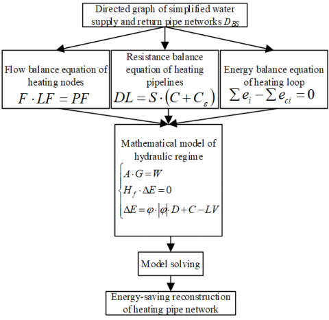
Figure 2. Mathematical model of the hydraulic regime of the simplified system
Figure 2 presents the mathematical model of the hydraulic regime of the simplified system. Suppose the incoming and outgoing flows at any heating node in the water supply and return network of the ICH system are negative and positive, respectively. According to the law of conservation of mass, the sum of positive and negative flows is zero. Let NI be the number of independent heating pipelines in the water supply and return network; NA be the number of associated heating nodes; F be the (NA-1)×NI-dimensional incidence matrix of the heating pipelines; LF=(LF1, LF2, …, LFNI)T be the column vectors of the flows in heating pipelines; PF=(PF1, PF2, …, PFNA)T be the column vectors of the flows at heating nodes. Then, the flow matrix of each heating node in the water supply and return network can be described by:
$F \cdot L F=P F$ (6)
When there is not fault pipeline in the water supply and return network, PF is a zero vector, i.e., PF=(0, 0, …, 0)T.
In the concentrated heating pipe network, energy loss may occur as the fluid rubs the pipe walls, and passes through pipeline accessories (where the flow state suddenly changes). Let DLb and ∑DLi be the frictional losses along the heating pipeline and in local areas, respectively; S be the loss per unit distance. Then, the frictional loss DL of a pipeline of the length C can be expressed as:
$D L=D L_{b}+\Sigma D L_{i}=S \cdot C+\Sigma D L_{i}$ (7)
where, DLb can be calculated by:
$D L_{b}=S \cdot C$ (8)
Let μ be the frictional coefficient between pipe walls and hot water; ε be the inner diameter of pipeline; σ and υ be the density and flow velocity of hot water, respectively. Then, the specific frictional resistance of heating pipeline can be calculated based on the Darcy–Weisbach equation:
$S=\frac{\mu}{\varepsilon} \cdot \frac{\sigma v^{2}}{2}$ (9)
The value of μ depends on the flow state of the hot water in the heating pipeline, and the smoothness of the pipe walls. Suppose the hot water is in a turbulent flow state. The μ value of a heating pipeline with an inner diameter <40mm can be derived by the Nikuradse empirical formula:
$\mu=\frac{1}{\left(1.14+2.1 g \frac{\varepsilon}{\Phi}\right)^{2}}$ (10)
If the inner diameter is greater than 40mm, the μ value can be computed by the Щuфрuнсон formula:
$\mu=0.11 \cdot\left(\frac{\Phi}{\varepsilon}+\frac{68}{R e}\right)^{0.25}$ (11)
where, Re is the Reynolds number of hot water flowing in the pipeline. The value of Φ differs from indoor to outdoor cases. In the outdoor case, the Φ value equals 5*10-4. In the indoor case, the Φ value equals 2*10-4. Let ∑δ be the sum of local resistance coefficients of a heating pipeline. Then, DLi can be calculated by:
$\Sigma D L_{i}=\sum \delta \cdot \frac{\sigma v^{2}}{2}$ (12)
During the calculation, ∑DLi can be substituted by frictional loss along the pipeline based on the equivalent length method. Then, the corresponding pipeline length can be calculated by:
$C_{\varepsilon}=\sum \delta \cdot \frac{\varepsilon}{\mu}=9 \cdot \varepsilon^{\frac{5}{4}} \cdot \sum \delta / \Phi^{\frac{1}{4}}$ (13)
Then, DL can be described by:
$D L=S \cdot\left(C+C_{\varepsilon}\right)$ (14)
When the hot water in the outdoor heating pipe network is a turbulent flow, DL is positively proportional to the square of hot water flow w. The proportionality coefficient can be denoted as φ. Then, DL can be calculated by:
$D L=S \cdot\left(C+C_{\varepsilon}\right)=\phi \cdot w^{2}=R C \cdot\left(C+C_{\varepsilon}\right) \cdot w^{2}$ (15)
The resistance characteristic coefficient φ of the heating pipe network can be calculated by:
$\phi=\frac{6.9 \cdot 10^{-9} \cdot \Phi^{\frac{1}{4}}}{\sigma \cdot \varepsilon^{5 \frac{1}{4}}}$ (16)
The resistance characteristic coefficient per unit length of the heating pipeline can be calculated by:
$R C=\frac{6.9 \cdot 10^{-9} \cdot \Phi^{\frac{1}{4}}\left(C+C_{\varepsilon}\right)}{\sigma \cdot \varepsilon^{5 \frac{1}{4}}}$ (17)
To drive the continuous flow of hot water in the pipeline, circulating water pumps should be arranged in the community heating system. Apart from the pressure of the circulating water pumps, the elevation difference could affect the pressure difference between two heating nodes. Let USOi and USFi be the start and end points of the i-th pipe segment in the hot water flow direction, respectively; EDi and eci be the elevation difference between the two points, and lift of circulation water pumps, respectively. Suppose the ec in the heating pipeline without circulating water pumps equals zero. Then, the pressure difference between two heating nodes can be calculated by:
$U S_{F \bar{i}}-U S_{O i}=e_{i}+E D_{i}-e_{c i}$ (18)
In the community heating system, the pressure drop equation of the heating loop, i.e., the energy balance equation of the heating loop, can be characterized by:
$\sum e_{i}-\Sigma e_{c i}=0$ (19)
From formula (19), it can be seen that the sum of the lifts of circulating water pumps in the closed heating loop equals the sum of the pressure losses in each pipe segments. That is, the algebraic sum equals zero.
During the IoT-based energy-saving reconstruction of community heating system, the water supply pipeline and water return pipeline might be out of sync in terms of hot water temperature, and water flow velocity, owing to the disparity of pipe materials and construction techniques. Suppose the incidence matrix F about the topological relationship between heating nodes and heating pipeline has a rank of (NA-1), and a size of NA-1)×NI. Then, the basic loop matrix with a rank of (H-NA+1), and a size of (H-NA+1)×S can be denoted as H, which equals the number of pressure drop equations in the heating loop. Let φ be the diagonal matrix of the frictional characteristic coefficients of heating pipelines; |D| be the combined vector of heating node flows; LV be the lift vectors of circulating water pumps. Then, a more realistic model can be constructed for the hydraulic regime in water supply pipeline and water return pipeline, respectively:
$\left\{\begin{array}{l}A \cdot G=W \\ H_{f} \cdot \Delta E=0 \\ \Delta E=\phi \cdot|\phi| \cdot D+C-L V\end{array}\right.$ (20)
Comparing the dimensionalities and ranks of different matrices, the above model has a unique solution.
2.3 Analysis of heating pipe network reconstruction
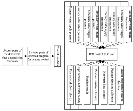
Figure 3. IoT-based monitoring of community heating pipe network
Figure 4. Control variables of heating system
Figure 3 illustrates the monitoring requirements of the IoT-based community heating system. For energy-saving reconstruction of community heating system, it is necessary to re-evaluate the hydraulic balance state of the heating pipe network in the community, replace the pipelines whose sizes are unsuitable, and add circulating water pumps to the pipelines with insufficient circulation power. In addition, indoor temperature sensors, pipeline temperature sensors, pipeline pressure sensors, and water flow velocity testers should be added to collect the real-time heating data. Meanwhile, a hydraulic balance master control valve should be deployed at the hot water inlet of each building in the community; a hydraulic balance branch control valve should be added to the hot water inlet on each floor in each building. The data should be collected in real time, and remotely transmitted to the remote monitoring center of community heating. Then, the hydraulic balance solenoid values would be regulated automatically, such that the indoor heating effect reaches the local standards. The above strategy of energy-saving reconstruction can counter the hydraulic and thermodynamic fluctuations at different periods in the community, and satisfy the stable operations of the system. The IoT-based technology helps the system to automatically adjust to the changes of external temperature.
After energy-saving reconstruction, the hydraulic situation of the community heating system was checked again. The results show that the hydraulic unbalance rate of the heating nodes was effectively reduced, and the change range of [5.6, 8.5] meets the requirement on hydraulic unbalance rate of community hot water supply. As a result, the heat demands between different layers of each building are well balanced.
The wireless data transmission terminals, which are responsible for collecting real-time data, were configured as follows: devices were added to and communication protocols were defined for the monitoring platform server; the serial ports were configured to read and write the field data of programmable logic controller (PLC). Figure 4 presents the control variables of heating system, and displays the structural relationship between modules.
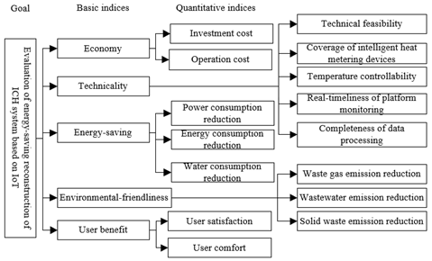
After energy-saving reconstruction, the community heating system was changed in operating model and heating control. The indoor temperature control was replaced with dual control of temperature and flow. When the outdoor temperature drops, the water supply temperature increases, and the flow of circulating hot water rises in the heating system. Under the dual control model, thermal mis-adjustment will not occur in the community under the optimal working condition, the thermal working state will remain stable, and the flow of circulating hot water will change adaptively to outdoor temperature. In this way, the electricity consumption will be reduced effectively. Figure 5 provides the evaluation indices of energy-saving reconstruction for IoT-based heating system. Some important quantifiable indices are simulated below.
Figure 5. Evaluation indices of energy-saving reconstruction for IoT-based heating system
Let τm be the goal of indoor temperature control; τH be the temperature in a place outdoor during heating; RF* be the ratio of actual flow RF to preset flow RF* of circulating water pump; HLR* be the relative heat load ratio of heating; θ be the flow optimization adjustment coefficient. Then, the preset flow can be calculated by:
$R F^{*}=\left(H L R^{*}\right)^{\theta}=\frac{R F}{R F^{\prime}}=\left(\frac{\tau_{m}-\tau_{H}}{\tau_{m}-\tau_{H}^{\prime}}\right)^{\theta}$ (21)
Let τO and τW be the water temperatures of water supply pipeline and water return pipeline, respectively, without energy-saving control; τ'O and τ'W be the water temperatures of water supply pipeline and water return pipeline, respectively, under energy-saving control; ω be the heating attribute coefficient of the radiator. Then, the optimal heating control method for community heating system after energy-saving reconstruction can be described by:
$\tau_{O}=\tau_{m}+\frac{1}{2}\left(\tau_{0}^{\prime}+\tau_{m}^{\prime}-2 \tau_{m}^{\prime}\right) \times\left(\frac{\tau_{m}-\tau_{H}}{\tau_{m}-\tau_{H}^{\prime}}\right)^{1 /(1+\omega)}$$+\frac{1}{2}\left(\tau_{o}^{\prime}-\tau_{m}^{\prime}\right) \times\left(\frac{\tau_{m}-\tau_{H}}{\tau_{m}-\tau_{H}^{\prime}}\right)^{1-\theta}$ (22)
$\tau_{O}=\tau_{m}+\frac{1}{2}\left(\tau_{o}^{\prime}+\tau_{m}^{\prime}-2 \tau_{m}^{\prime}\right) \times\left(\frac{\tau_{m}-\tau_{H}}{\tau_{m}-\tau_{H}^{\prime}}\right)^{1 /(1+\omega)}$$-\frac{1}{2}\left(\tau_{o}^{\prime}-\tau_{m}^{\prime}\right) \times\left(\frac{\tau_{m}-\tau_{H}}{\tau_{m}-\tau_{H}^{\prime}}\right)^{1-\theta}$ (23)
Formulas (22) and (23) show that, when the energy-saving reconstruction conditions are constant for community heating system, it is important to ensure the uniqueness of the temperature and flow adjustment values during the vertical disorder of the thermal regime. Let HLR* be the relative heat load of heating supply. Then, θ can be calculated by:
$\theta=\frac{\lg R F^{*}}{\lg H L R^{*}}$ (24)
In general, the θ value of the primary heating pipe network of the community equals 1; the θ values of single pipeline and dual pipelines in the secondary pipe network equal ω/(1+ω), and 0.33, respectively. Under energy-saving control, the operating efficiency and lift of circulating water pumps could be denoted as ξ' and E', respectively; the number of continuous heating hours in the heating season could be denoted as p. Then, the power consumption PC of circulating water pumps under energy-saving control can be calculated by:
$P C=\frac{R F^{\prime} E^{\prime} p}{367 \xi^{\prime}}$ (25)
If τH<τH', the hot water flows at the preset flow RF' of energy-saving control, i.e., RF=RF'; If τH>τH' or τH<τOR, the hot water flows beneath the preset flow RF' of energy-saving control, i.e., RF<RF'. The sum of power consumptions under the two scenarios is the power consumption PC in the heating season.
Let PC1 and PC2 be the sums of power consumption under τH. w≥τH≥τH and τH<τH', respectively; RFi be the flow of hot water circulating in an outdoor temperature interval; τOR and ∆pi be the minimum temperature and duration of the temperature interval, respectively; ξi be the operating efficiency of the circulating water pump; E be the control pressure difference of the pipeline; p0 be the duration of the preset outdoor temperature; pS be the duration of heating; p be the duration of an outdoor temperature. Then, PC can be calculated by:
$P C=P C_{1}+P C_{2}$$=\sum_{i=1}^{N_{I}} \frac{R F_{i} E \Delta p_{i}}{90 \xi_{i}}+\frac{R F^{\prime} E^{\prime} p_{0}}{90 \xi^{\prime}}$$=\frac{R F^{\prime}}{90 \xi^{\prime}} \sum_{i=1}^{N_{I}} \frac{R F_{i}\left(E_{G}+\frac{E^{\prime}}{R F^{\prime 2}} \times R F_{i}^{2}\right) \Delta p_{i}}{R F^{\prime}}$
$+\frac{R F^{\prime} E^{\prime} p_{0}}{90 \xi^{\prime}}$$=\frac{R F^{\prime}}{90 \xi^{\prime}} \sum_{i=1}^{N_{I}}\left(R F^{*} E+\left(R F^{*}\right)^{3} E^{\prime}\right) \Delta p_{i}+\frac{R F^{\prime} E^{\prime} p_{0}}{90 \xi^{\prime}}$$=\frac{R F^{\prime}}{90 \xi^{\prime}} \int_{p_{0}}^{p_{s}}\left(R F^{*} E+\left(R F^{*}\right)^{3} E^{\prime}\right) d p_{i}+\frac{R F^{\prime} E^{\prime} p_{0}}{90 \xi^{\prime}}$ (26)
Let τc be the mean outdoor temperature in the heating season; pC be the duration of outdoor temperature equal to or below τH; DGm be the set of dimensionless durations; DGτ be the set of dimensionless outdoor temperatures. Then, the temperature distribution law in the heating season can be described by DGm and DGτ:
$D G_{\tau}=\left\{\begin{array}{l}0 \quad p_{C} \leq 7 \\ D G_{m}^{\omega} \quad 7<p_{C} \leq p_{S}\end{array}\right.$ (27)
The law can also be described by:
$\tau_{H}=\left\{\begin{array}{lc}\tau_{H}^{\prime} & p_{C} \leq 7 \\ \tau_{H}^{\prime}+\left(7-\tau_{H}^{\prime}\right) D G_{m}^{\omega} & 7<p_{C} \leq p_{S}\end{array}\right.$ (28)
DGm, DGτ, ω and λ can be calculated by:
$D G_{m}=\frac{p_{C}-7}{p_{S}-7}, D G_{\tau}=\frac{\tau_{H}-\tau_{H}^{\prime}}{7-\tau_{H}^{\prime}}$ $\omega=7 \frac{5-\lambda \times \tau_{c}}{\lambda \times \tau_{c}-\tau_{H}^{\prime}}, \lambda=\frac{p_{S}}{p_{S}-7}$ (29)
Combining formulas (29) and (21):
$H L R^{*}=\left\{\begin{array}{lc}1 & p_{C} \leq 7 \\ 1-\alpha_{0} D G_{m}^{\omega} & 5<p_{C} \leq p_{S}\end{array}\right.$ (30)
where, α0 can be expressed by:
$\alpha_{0}=\frac{7-\tau_{H}^{\prime}}{\tau_{m}-\tau_{H}^{\prime}}$ (31)
For primary and secondary pipe networks, we have:
$R F^{*}=H L R^{*},\left(R F^{*}\right)^{3}=H L R^{*}$ (32)
After sorting, the power consumption of circulating water pumps in the primary pipe network can be described as:
$P C=P C_{1}+P C_{2}=$$\frac{R F^{\prime}}{90 \xi^{\prime}} \int_{p_{0}}^{p_{s}}\left\{\begin{array}{l}E\left[1-\frac{7-\tau_{H}^{\prime}}{\tau_{m}-\tau_{H}^{\prime}} \cdot\left(\frac{p_{C}-7}{p_{S}-7}\right)^{\omega}\right] \\ \left.+\left[1-\frac{7-\tau_{H}^{\prime}}{\tau_{m}-\tau_{H}^{\prime}} \cdot\left(\frac{p_{C}-7}{p_{S}-7}\right)^{\omega}\right]^{3}\right\}\end{array}\right\} d p$$+\frac{R F^{\prime} E^{\prime} p_{0}}{90 \xi^{\prime}}$ (33)
Similarly, the power consumption of circulating water pumps in the secondary pipe network can be sorted out as:
$P C=\frac{R F^{\prime}}{90 \xi^{\prime}} \int_{p_{0}}^{p_{s}}\left\{\begin{array}{l}E\left[1-\frac{7-\tau_{H}^{\prime}}{\tau_{m}-\tau_{H}^{\prime}} \cdot\left(\frac{p_{C}-7}{p_{S}-7}\right)^{6}\right]^{\frac{1}{3}} \\ +\left[1-\frac{7-\tau_{H}^{\prime}}{\tau_{m}-\tau_{H}^{\prime}} \cdot\left(\frac{p_{C}-7}{p_{S}-7}\right)^{6}\right]\end{array}\right\} d p$$+\frac{R F^{\prime} E^{\prime} p_{0}}{90 \xi^{\prime}}$ (34)
Let gBU be the thermal consumption of buildings in the community; gHN be amount of standard coal consumed for heating; STHN be the calorific value of standard coal; γ1 be the transmission efficiency of heat supply pipe network of the community; γ2 be the efficiency of the heat source. Then, the coal consumption of the community for heating after energy-saving reconstruction can be calculated by:Formula 34 shows that the power consumption of circulating water pumps is a univalent function of pC. The total power consumption of circulating water pumps in the heating period after energy-saving reconstruction can be calculated by substituting the real-time data collected by IoT monitoring system (e.g., thermal exchanger parameters and circulating water pump efficiencies of primary and secondary pipe networks) into formula 34.
$g_{H N}=\frac{24 \cdot p_{S} \cdot g_{B U}}{S T_{H N} \cdot \gamma_{1} \cdot \gamma_{2}}$ (35)
Table 1 lists the hydraulic balance results of community heating system during the IoT-based energy-saving reconstruction.
Table 1. Hydraulic conditions of system loops before energy-saving reconstruction
|
Serial number |
Load |
Flow |
Pipe diameter |
Pipe length |
υ |
S |
Dynamic pressure |
Pipeline frictional loss |
|
1 |
445 |
15352.8 |
DN100 |
120 |
0.495 |
27.963 |
118.775 |
3215.367 |
|
2 |
445 |
15352.8 |
DN100 |
15 |
0.491 |
27.963 |
118.775 |
375.752 |
|
3 |
882 |
31712.1 |
DN130 |
261 |
0.643 |
35.251 |
207.021 |
9572.341 |
|
4 |
385 |
13525 |
DN90 |
75 |
0.742 |
87.128 |
273.672 |
7176.213 |
|
5 |
385 |
13532 |
DN90 |
32 |
0.742 |
87.128 |
273.672 |
2571.318 |
|
6 |
760 |
26718 |
DN110 |
127 |
0.854 |
82.351 |
375.128 |
13172.051 |
|
7 |
479 |
16351.9 |
DN110 |
85 |
0.526 |
31.972 |
134.875 |
2671.389 |
|
8 |
479 |
16351.9 |
DN110 |
49 |
0.526 |
31.972 |
135.729 |
1767.428 |
|
9 |
973 |
32547.3 |
DN130 |
15 |
0.679 |
40.075 |
275.671 |
3276.84 |
|
10 |
1425 |
16584.2 |
DN110 |
103 |
0.520 |
30.784 |
523.487 |
473.592 |
|
Total |
7607 |
262993.5 |
|
1017 |
|
|
|
54105.337 |
Table 2. Indoor temperatures before and after energy-saving reconstruction
|
Building number |
Pre-reconstruction |
Post-reconstruction |
|
1# |
15 |
18 |
|
2# |
13 |
19 |
|
3# |
22 |
22 |
|
4# |
19 |
20 |
|
5# |
17 |
18 |
|
6# |
16 |
18 |
|
7# |
19 |
25 |
|
8# |
12 |
19 |
|
9# |
14 |
19 |
|
10# |
17 |
24 |
Figure 6. Temperature and flow changes of primary pipe network
Before energy-saving reconstruction, the buildings, except for buildings 3#, 4#, and 7#, did not reach the standard indoor temperature of 18℃ during the heating season. After the IoT-based energy-saving reconstruction, the indoor temperature of all buildings in the community increased greatly, surpassing 18℃. The indoor thermal comfort, and heat supply quality both improved (Table 2).
Figure 6 presents the temperature and flow changes of primary pipe network after energy-saving reconstruction. When the outdoor temperature remained the same, the temperature of the water supplied by the heat source changed in the range of [6, 12], and that of water return pipeline changed within [5, 10]. Therefore, the water supply and return of the primary pipe network are controlled with a high precision. In addition, the hot water flow, which changed in [5, 8], also fell in the ideal control range.
Figure 7. Variation of system energy consumption with outdoor temperatures
Figure 7 shows how the energy consumption of community heating system changed with outdoor temperature. It can be seen that the energy saved by the heat source of the system fluctuated very slightly, but the water consumption, which is loosely coupled with outdoor temperature, oscillated greatly. The coal consumption for heating, which is strongly associated with outdoor temperature, was relatively loosely controlled. Under the same outdoor temperature, there was a 16.5% difference of coal consumption. Therefore, the control of coal consumption should be further improved.
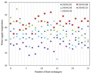
Figure 8. Variation in water supply temperature of heat exchangers in the secondary pipe network
Figure 8 shows the variation in water supply temperature of heat exchangers in the secondary pipe network of the community heating system during the heating season of 2019. Almost all heat exchangers operated with a large flow and a small temperature difference. The temperature difference fluctuated in [2, 5]. The actual flow of circulating hot water was about 1.14 times of the preset flow. Figure 9 records the utilizable pressure head of heat exchangers in the secondary pipe network. To a certain extent, the utilizable pressure head reflects the flow and power of hot water circulation in the system. As shown in Figure 9, the utilizable pressure head of heat exchangers changed within [0.05, 0.14], which is within the ideal controllable range. Table 3 provides the specific operating data of heat exchangers.
Figure 9. Variation in utilizable pressure head of heat exchangers in secondary pipe network
The total heating energy reduction of the community consists of three parts: coal consumption reduction, power consumption reduction of the heat source, primary pipe network, and secondary pipe network, and water consumption reduction of primary and secondary pipe networks. Tables 4 and 5 display the coal consumption reduction and power consumption reduction in different heating seasons, which were calculated based on the measured data in these seasons before and after energy-saving reconstruction.
As shown in Tables 4 and 5, the energy-saving reconstruction effectively suppressed the actual coal consumption of the heat source in the community heating system. The coal consumption indices dropped from 30.35 and 31.47 before the reconstruction to 30.72 and 29.63 after the reconstruction. Without considering the power consumed by the environmentally-friendly measure of desulfurization, the heat source, heat exchangers, and the system saved 33.98%, 17.93%, and 7.52% of power, respectively. The primary and secondary pipe networks consumed a total of 2.54kWh/m2 of power, about 24.13% lower than the pre-reconstruction power consumption.
Table 3. Operating data of heat exchangers
|
Serial number of heat exchangers |
Primary water supply pipe network |
Primary water return pipe network |
Secondary water supply pipe network |
Secondary water return pipe network |
||||
|
Pressure |
Temperature |
Pressure |
Temperature |
Pressure |
Temperature |
Pressure |
Temperature |
|
|
1# |
0.57 |
65 |
0.57 |
38 |
0.27 |
35 |
0.21 |
35 |
|
2# |
0.63 |
72 |
0.62 |
36 |
0.35 |
43 |
0.23 |
37 |
|
3# |
0.72 |
69 |
0.69 |
37 |
0.36 |
41 |
0.25 |
39 |
|
4# |
0.61 |
63 |
0.64 |
41 |
0.27 |
45 |
0.27 |
32 |
|
5# |
0.43 |
65 |
0.38 |
42 |
0.42 |
40 |
0.26 |
32 |
|
6# |
0.89 |
62 |
0.76 |
41 |
0.35 |
43 |
0.35 |
36 |
|
7# |
0.68 |
68 |
0.65 |
35 |
0.34 |
41 |
0.31 |
36 |
|
8# |
0.72 |
53 |
0.62 |
36 |
0.25 |
36 |
0.27 |
31 |
|
9# |
0.23 |
67 |
0.25 |
35 |
0.29 |
38 |
0.26 |
35 |
Table 4. Coal consumption reduction in different heating seasons
|
Year |
Actual heating area |
Mean outdoor temperature |
Mean indoor temperature |
Coal consumption of heat source |
Coal consumption index |
Remark |
|
2015-2016 |
1823100 |
-6.5 |
17.84 |
57120 |
30.35 |
Pre-consumption |
|
2016-2017 |
1804900 |
-6.32 |
17.23 |
54360 |
31.47 |
Pre-consumption |
|
2017-2018 |
1807520 |
-5.21 |
19.95 |
53375 |
30.72 |
Post-consumption |
|
2018-2019 |
1879160 |
-5.67 |
18.27 |
53621 |
29.63 |
Post-consumption |
Table 5. Power consumption reduction in different heating seasons
|
Year |
Heat source |
Heat exchangers |
System |
|||
|
Power consumption |
Power consumption index |
Power consumption |
Power consumption index |
Power consumption |
Power consumption index |
|
|
2015-2016 |
112350 |
1.35 |
2971252 |
1.55 |
4712012 |
2.65 |
|
2016-2017 |
935452 |
1.89 |
2871423 |
1.58 |
4516276 |
2.55 |
|
2017-2018 |
452125 |
0.95 |
2854987 |
1.52 |
4372318 |
2.45 |
|
2018-2019 |
632510 |
1.23 |
2781565 |
1.44 |
4395293 |
2.49 |
|
Node proportion % |
-725.12 |
33.98 |
16.47 |
17.93 |
6.35 |
7.52 |
Table 6. Emission reduction of different pollutants
|
Item |
Waste gas emissions |
Wastewater emissions |
Solid waste emissions |
|
Pre-reconstruction |
27.41 |
20.35 |
14.71 |
|
Post-reconstruction |
25.13 |
19.23 |
13.52 |
|
Emission reduction |
2.28 |
1.12 |
1.19 |
Before and after the reconstruction, the community heating system always adopts gas-fired boilers. Table 6 presents the changes in the emission reduction of main pollutants. The emissions of waste gas declined by 2.28kg from 27.41kg before the reconstruction to 25.13kg after the reconstruction. The emissions of wastewater dropped by 1.12 tons from 20.35kg before the reconstruction to 19.23 tons after the reconstruction. The emissions of solid waste decreased by 1.19 tons from 14.71 tons before the reconstruction to 13.52 tons after the reconstruction.
This paper researches and evaluates the energy-saving reconstruction of IoT-based ICH system. Firstly, the water supply and return networks were simplified, and a mathematical model was built up for the hydraulic regime of the simplified system. Next, the authors constructed the equations of node flow balance, pipeline pressure drop balance, and loop pressure drop balance, and finalized the mathematical model of the hydraulic regime of the system. After that, the energy consumptions of the system before and after energy-saving reconstruction were detailed, and the energy-saving benefit of the system was predicted accurately. Finally, multiple parameters of the system, i.e., indoor temperature, water supply temperature, water supply flow, utilizable pressure head, and operating data of heat exchangers, were compared through experiments. The comparison verifies the effectiveness of our energy-saving reconstruction plan. In addition, the energy consumption reduction in multiple heating seasons was recorded before and after the reconstruction.
This paper was supported by the Fundamental Research Funds for the Central Universities (Grant No.: ZY20210301); Langfang science and technology research self-funded project (Grant No.: 2021011020).
[1] Shi, H.X., An, W.T., Xu, D.T., Tian, Q.Y., Zhang, Z.H., Ren, Y.K., Ouyang, S. (2020). Regulation for energy-saving operation of energy supply system in plant factory with energy-storage ground-source heat pump. Nongye Gongcheng Xuebao/Transactions of the Chinese Society of Agricultural Engineering, 36(1): 245-251.
[2] Wong, K.J., Shih, S.H., Shih, Y.C., Chao, L.Y., Cho, J.F., Huang, X.L. (2018). The energy-saving effect of installing a heat recovery ventilatior on a residence house. ACRA 2018 - 9th Asian Conference on Refrigeration and Air-Conditioning.
[3] Wang, L., Dong, Y., Zhou, S.H., Chen, E., Tang, S.W. (2018). Energy saving benefit, mechanical performance, volume stabilities, hydration properties and products of low heat cement-based materials. Energy and Buildings, 170: 157-169. https://doi.org/10.1016/j.enbuild.2018.04.015
[4] Chen, T., Cai, L. (2018). Energy-saving analysis of a hybrid-power gas engine heat pump with continuously variable transmission. International Energy Journal, 18(4).
[5] Zhao, J., Wang, R., Wang, M., Huang, X. (2019). Application of heat pump energy-saving flue-cured tobacco technology. In IOP Conference Series: Earth and Environmental Science, 252(3): 032042.
[6] Wang, M.Z., Ren, F.J., Zang, J.J., Chen, Z.P., Hao, W., Zhang, X.X., Liu, J.J. (2019). Environmental control and energy saving effect of heat lamp with variable power heating for piglets. Nongye Gongcheng Xuebao/Transactions of the Chinese Society of Agricultural Engineering, 35(15): 182-191.
[7] Kunitomo, O., Satoh, I., Hiroshima, M. (2019). Reduction of conveyance power consumption of district cooling and heating systems using demand-supply coordinated control-part 2-energy saving effect of demand-supply coordinated control system. In E3S Web of Conferences, 111: 06008. https://doi.org/10.1051/e3sconf/201911106008
[8] Zakharov, V.M., Smirnov, N.N., Tyutikov, V.V., Flament, B. (2015). Energy efficiency by use of automated energy-saving windows with heat-reflective screens and solar battery for power supply systems of European and Russian buildings. In IOP Conference Series: Materials Science and Engineering, 93(1): 012015.
[9] Cooper, S.J., Hammond, G.P., Hewitt, N., Norman, J.B., Tassou, S.A., Youssef, W. (2019). Energy saving potential of high temperature heat pumps in the UK food and drink sector. Energy Procedia, 161: 142-149. https://doi.org/10.1016/j.egypro.2019.02.073
[10] Trafczynski, M., Markowski, M., Urbaniec, K. (2019). Energy saving potential of a simple control strategy for heat exchanger network operation under fouling conditions. Renewable and Sustainable Energy Reviews, 111: 355-364. https://doi.org/10.1016/j.rser.2019.05.046
[11] Eom, Y.H., Yoo, J.W., Hong, S.B., Kim, M. S. (2019). Refrigerant charge fault detection method of air source heat pump system using convolutional neural network for energy saving. Energy, 187: 115877. https://doi.org/10.1016/j.energy.2019.115877
[12] Chen, D.L., Zhang, Z.L., Yang, J.X. (2019). Process simulation and energy saving analysis of CO2 capture by chemical absorption method based on self-heat recuperation. CIESC Journal, 70(8): 2938-2945.
[13] Shalaginova, Z.I. (2014). Estimating the energy saving potential from carrying out adjustment works in heat supply systems on the basis of modeling their thermal-hydraulic operating modes. Thermal Engineering, 61(11): 829-835. https://doi.org/10.1134/S0040601514090109
[14] Kobzar, A.V., Babenko, G.S., Turchanovich, N.N. (2017). Performance potential of energy savings using solar energy in heat supply systems for buildings in the primorsky krai. In 2017 International Conference on Industrial Engineering, Applications and Manufacturing (ICIEAM), pp. 1-6. https://doi.org/10.1109/ICIEAM.2017.8076270
[15] Abdelaziz, G.B., Abdelbaky, M.A., Halim, M.A., Omara, M.E., Elkhaldy, I.A., Abdullah, A.S., Kabeel, A.E. (2021). Energy saving via heat pipe heat exchanger in air conditioning applications “experimental study and economic analysis”. Journal of Building Engineering, 35: 102053. https://doi.org/10.1016/j.jobe.2020.102053
[16] Hwang, Y.J., Jeong, J.W. (2021). Energy saving potential of radiant floor heating assisted by an air source heat pump in residential buildings. Energies, 14(5): 1321. https://doi.org/10.3390/en14051321
[17] Watanabe, N., Mizutani, T., Nagano, H. (2021). High-performance energy-saving miniature loop heat pipe for cooling compact power semiconductors. Energy Conversion and Management, 236: 114081. https://doi.org/10.1016/j.enconman.2021.114081
[18] Luo, Q.H., Zuo, Z. (2012). Heat pumps for energy saving of building hot water supply. In Advanced Materials Research, 347: 587-590. https://doi.org/10.4028/www.scientific.net/AMR.347-353.587
[19] Malakhov, V.A. (2012). Assessing the economic effect from introduction of energy-saving technologies in the field of heat supply. Thermal Engineering, 59(3): 250-257. https://doi.org/10.1134/S0040601512030093
[20] McBrien, M., Serrenho, A.C., Allwood, J.M. (2016). Potential for energy savings by heat recovery in an integrated steel supply chain. Applied Thermal Engineering, 103: 592-606. https://doi.org/10.1016/j.applthermaleng.2016.04.099
[21] Tang, L., Xing, Y.L. (2013). Energy-saving optimization of heating supply systems of Sino-Singapore (Tianjin) eco-city energy planning. In Advanced Materials Research, 689: 453-458. https://doi.org/10.4028/www.scientific.net/AMR.689.453
[22] Long, J., Xia, K., Zhong, H., Lu, H., Yongga, A. (2021). Study on energy-saving operation of a combined heating system of solar hot water and air source heat pump. Energy Conversion and Management, 229: 113624. https://doi.org/10.1016/j.enconman.2020.113624
[23] Sun, L., Yang, M.D., Luo, X.L. (2020). Slow-release optimization of heat exchange networks based on sustainable energy saving. Huagong Jinzhan/Chemical Industry and Engineering Progress, 39(10): 3941-3948.
[24] Dongellini, M., Naldi, C., Morini, G.L. (2021). Influence of sizing strategy and control rules on the energy saving potential of heat pump hybrid systems in a residential building. Energy Conversion and Management, 235: 114022. https://doi.org/10.1016/j.enconman.2021.114022
[25] Muneeshwaran, M., Wang, C.C. (2021). Energy-saving of air-cooling heat exchangers operating under wet conditions with the help of superhydrophobic coating. Energy Conversion and Management, 229: 113740. https://doi.org/10.1016/j.enconman.2020.113740
[26] Marshalova, G.S., Sukhotskii, A.B., Kuntysh, V.B. (2020). Enhancing energy saving in air cooling devices by intensifying external heat transfer. Chemical and Petroleum Engineering, 56: 85-92. https://doi.org/10.1007/s10556-020-00743-6
[27] Takeda, T., Okazawa, R. (2020). Study on energy saving effect of ground source heat pump applied as greenhouse air conditioning system. ICOPE 2019 - 7th International Conference on Power Engineering, Proceedings, pp. 425-429.
[28] Zanetti, E., Aprile, M., Kum, D., Scoccia, R., Motta, M. (2020). Energy saving potentials of a photovoltaic assisted heat pump for hybrid building heating system via optimal control. Journal of Building Engineering, 27: 100854.