Veyan A. Musa* | Raid A. Mahmood | Shwan M. Noori Khalifa | Omar M. Ali | Lokman A. Abdulkareem
© 2021 IIETA. This article is published by IIETA and is licensed under the CC BY 4.0 license (http://creativecommons.org/licenses/by/4.0/).
OPEN ACCESS
The current investigation aimed to identify pressure gradients and to study the fully developed flow patterns of oil-gas as a blend in a pipe of internal diameter 50 mm and 6 m length with different orientations of 0, 30, and 45-degree. The study was performed at constant values of liquid superficial velocities 0.052, 0.157, 0.262, 0.314, 0.419, and 0.524 m/s, and inlet superficial velocities of gas were ranged from 0.05 to 4.7 m/s at atmospheric pressure. Two pressure transducers located up and downstream were used to measure pressure drops inside the tested pipe. Flow patterns were derived by using the correlation between pressure gradients and time series, the Probability Density Function of differential pressures, pressure gradients with gas superficial velocities, and total pressure losses with mean void fractions. The flow patterns of oil-gas were observed as a uniform stratified flow in the pipe on a 0-degree orientation at various superficial velocities. Stratified, wavy, and slug flow patterns were observed at 30-degree orientation, whereas, bubbly, slug, and churn flow patterns were observed in the pipe of 45-degree orientation. The experiment also showed that pressure drop gradients decreased with increased void fractions, gas superficial velocities, and degree rotations of the flow lines. Finally, the validation of using pressure transducers as a technique for estimating the flow patterns of two-phase flow showed acceptable results with some kind of patterns.
pressure drops in the two-phase flow, two-phase flow patterns in pipes, oil-gas flow patterns, differential pressure transducers
Oil-gas two-phase flow plays an important role in various engineering and industry applications such as in pipelines and power generation plants [1]. However, two-phase flow is a very complicated and complex flow compared with single-phase flow. Pressure drop is one of the complex issues in two-phase flow as it is affected by flow pattern, geometry, and operating conditions. The investigations of pressure drop in the two-phase flow required considering parameters and circumstances that influence the flow. However, the total pressure drops produced by the process of two-phase flow transportation in pipes are presenting an attractive and very important factor in designing effective systems. Pressure drops are participating in calculations of energy conservation of any system. Moreover, other factors, such as pipes orientation and flow direction also have an enormous impact on the structure of two-phase flow which is manifested in the flow in terms of spatial and geometrical distribution which is called flow patterns. Those parameters are extremely important as they determine the estimation of the properties of the operating systems [2].
Theoretically, there is no reliable method that can be used to predict pressure drops of two-phase flow accurately due to the nonlinear behavior that this flow conducted [3, 4]. The inversion phenomena between both phases complicate the issue furthermore and this causes the prediction of pressure drop more challenging [5]. From the literature, a pressure drop significantly increases at the inversion point of phases [6]. However, the first homogenous model of two-phase flow is estimated from the model which was presented by Brinkman [7], after many studies used the same model such as Angeli and Hewitt [6], who applied the Brinkman’s model with a considerably high ratio of uncertainty in results. Picchi et al. [8] created another two-phase flow model depended on the assumption of merely one of the two phases should not be generalized, since it has not been validated on generic models with a point of phase inversion.
The two-phase experimental investigation of pressure drops that occurred in pipes by using specific methods for analyzing the obtained data such as Power Spectral Density (PSD), Probability Density Function (PDF), and void fractions analysis is more reasonable and reliable. The investigation in fluctuation produced by the flow of air-water inside a horizontal pipe was started by Hubbard [9], they obtained a method to identify flow patterns utilizing PSD correlation with frequencies, they optimized dispersed or bubbly flow at a constant frequency, and stratified flow pattern is characterized under maximum PSD at zero frequency.
Jones and Zuber [10] have been pioneered the photon attenuation procedure to quantify the relationship between time series and cross-sectional void fractions to investigate the flow patterns of air and water in a vertical pipe, the possibility of using the PDF as a method to describe flow regimes has been confirmed. Taitel et al. [11] studied the flow patterns of air and water inside a vertical pipe of an internal diameter of 50 mm, they showed that bubbly flow pattern occurred when the void fraction of flow is equal to or less than 0.25, but the flow pattern would then change to plug regime with increasing the value of void fraction because the small bubbles will be gathering and then the flow regime transits to plug flow, also an equation showed the relationship between the two phases velocities was arrived as followed [11]:
$\mathrm{U}_{\mathrm{sl}}=\left(3 \times \mathrm{U}_{\mathrm{sg}}\right)-1.15 \times\left[\frac{\sigma \mathrm{g}\left(\rho_{\mathrm{liq}}-\rho_{\mathrm{gas}}\right)}{\rho_{\mathrm{liq}}{ }^{2}}\right]^{0.25}$. (1)
Perez [12] used Electrical Capacitance Tomography (ECT) as a sensor to obtain the flow patterns of air-water in two pipes of internal diameters 38 and 67 mm at different orientations. The researcher investigated the impact of the pipe angular position on the flow distribution. The author depicted that slug flow was the dominant pattern for most tests of the near to vertical position comparing with the stratified flow regime in the horizontal flow pipelines. Also, he studied the impact of the inclination angle and air superficial velocities on pressure drop. Abdulkareem et al. [13] as a part of his study, investigated the flow regimes of silicone oil-gas that occurred in a pipe of internal diameter 67 mm with various orientation angles ranging from 0 to 90 degrees. He used three devices as sensors; A WMS, ECT, and Differential Pressure Transducer (DPT), the results have been concluded by analyzed PDF, liquid holdups in the domain of time series, and PSD to identify the flow patterns, as well as, he classified the flow patterns as a bubbly, stratified-wavy, slug flow in a pipe with that orientation angles less than 45-degree whereas, the churn flow pattern is estimated in a pipe of rotations equal and more than 45-degree.
A study of utilizing the differential values of pressure to estimate the void fractions of air-water flow has been carried out by Jia et al. [14] in a horizontal pipe. A Wire-Mesh Sensor (WMS) and an Electrical Resistance Tomography (ERT) have been utilized as sensors to validate the calculation of void fractions analytically. They obtained a reasonable comparison between the experimental results recorded from the two sensors and the equation, however, the calculated Eqns. (2) and (3) are shown below.
$\alpha=1-\frac{\Delta p}{\rho_{l i q} h}+\frac{2 C_{f} v^{2}}{g D}$, (2)
$\mathrm{C}_{\mathrm{f}}=0.079 \mathrm{Re}^{-0.25}$. (3)
Da Salve et al. [15] studied the flow regimes of air-water flow in a horizontal flowline of an internal diameter of 19.5 mm, and they classified the flow patterns as stratified, plug, slug, and annular utilizing the analysis methods of PDF, the void fraction of time series, and PSD. Hanafizadeh et al. [16] examined the flow patterns of water-oil in an inclined pipe of the rotation ranged from -45 to +45 degrees with an internal diameter of 20 mm using a high-speed camera. The authors estimated a flow regime map for each pipe position and they compared their results with other previous researches, besides, they observed bubbly, slug, stratified, wavy-stratified, annular and churn flow patterns in the different pipe orientations.
A study was conducted by Yao et al. [17] to evaluate the frictional pressure drop in a vertical downflow air-water mixture at room temperature in different pipe's internal diameters of 15, 25, 40, and 40 mm. they concluded that buoyancy force can push to raise the frictional pressure drop of the flow, and they obtained a new model predicts frictional pressure losses in a vertical pipe with an acceptable result. Musa et al. [18] carried out a study in air-water flow to investigate flow patterns in a horizontal and vertical pipe of an internal diameter 67 mm at different superficial velocities of both phases by using the following methods: PDF, PSD, tomography images, and the void fractions of time series to estimate the patterns have occurred in the mentioned pipe, the flow patterns in the vertical pipe were classified as bubbly flow patterns at lower values of air superficial velocities; slug flow at moderate air superficial velocities; and churn flow at a considerably higher flow rate of air.
Wen et al. [19] Studied the best performing model that could be present the void fractions of two-phase flow in inclined pipe ranged from 0 to 30 degrees of an internal diameter 75 mm. they examined six models by considering the flow mixture type, pipe diameter, and the orientation of the pipe. The correlation of modified-Hughmark [20] gave the best accuracy with the small orientation angle in the horizontal direction of air-water flow, while the model of Beggs-Brill [21] presented more accuracy with a flow consist of white oil and air.
Baghernejad et al. [22] investigated the effect of inclination on pressure losses of air-water in a pipe of internal diameter 25.4 mm, and length of 4 m. The results of their experiment revealed that the inclination angle of the utilized pipe has a significant impact on pressure drops, they also dictated that the level of water in the horizontal pipe reduced as the pipe inclination angle increased, when the stratified pattern generated. Additionally, they summed up that for both inclined and horizontal pipes, pressure losses significantly increased with increasing the pipe angle. Moreover, they investigated the effect of the increasing value of Usg on the pressure drop in the horizontal pipe and compared their results with other previous results from other studies.
Lately, many techniques were used in researches to identify the distribution of two-phase inside pipes at different orientations, like Wire-Mesh Sensor (WMS) [23, 24], X-ray Tomography [25]. However, the pressure drops in different orientations using oil-gas two-phase flow were not presented sufficiently. therefore, the objective of this study is to investigate the pressure drops that occurred in various pipe’s orientation degrees besides, the flow patterns of oil-gas flow. The possibility of classifying the patterns of two-phase flow with a minimum cost of value techniques like differential pressure transducers is studied in the current research, furthermore, this study will provide additional information about the distribution properties of oil-gas as a mixture in different condition for designers.
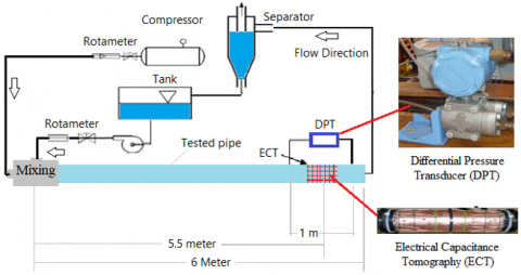
The present test was carried out at atmospheric pressure by utilizing an up-direction flow consisting of oil and gas in a pipe of an internal diameter of 50 mm. The experiment is performed at different superficial velocities of oil; 0.052, 0.157, 0.262, 0.314, 0.419, and 0.524 m/s with inlet superficial velocities of gas ranged from 0.05 to 4.7 m/s. The experiments were repeated under various pipe orientations; 0, 30, and 45-degree. A Differential Pressure Transducer (DPT) type; Rosemount 2024 DP cell was utilized to estimate the total pressure drops of one meter. ECT was jointed also at the end of the tested pipe with a distance of 5.5 m far from the mixing device as illustrated in Figure 1.
Figure 1. Experiment structure
The flow as a loop was injected into the tested pipe by an air compressor and water pump. The flow was mixed to enter the pipe and finally directed to a separator and storage tank. The storage water tank was used to maintain the temperature of the tested flow at a constant of 27℃.
Two-phase flow patterns were estimated by analyzing the data of mean void fractions (α) obtained by the Electrical Capacitance Tomography (ECT) sensor which was utilized in the current study as a non-intrusive technique. ECT sensor was based on capacitance measurements and it is used frequently by many researchers to obtain the void fractions (α) of the flow. More information about ECT is stated intensively in Ref. [26].
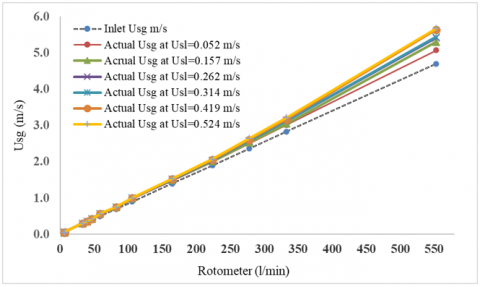
A correlation was conducted to calculate the actual values of Usg were impacted by the pressure produced inside the pipe which was considered as a prim uncertainty factor in such type of flow at various pipe inclinations as shown in Figure 2. The correlations were obtained by Eqns. (4) and (5) as derived by Abdulkareem [13].
$\mathrm{U}_{\mathrm{sg}}=\mathrm{m} / \rho_{\mathrm{p}} \mathrm{A}_{\mathrm{p}}$, (4)
$\mathrm{m}=\rho_{\mathrm{A}} \mathrm{Q} \sqrt{\rho_{\mathrm{R}}}$. (5)
where, $\rho_{P}$=1.2 Pp = Gas density at pipe pressure,
$\rho_{\mathrm{R}}$= gas density at reference (1.2),
$\rho_{\mathrm{A}}$= 1.2 PA = Gas density at different area mete,
PA is the pressure at different area meters.
The mean void fractions were estimated by utilizing the tomography ECT sensor, whereas the total and frictional pressure gradients are calculated using the following equations as adopted before in the study [13]:
$\frac{\mathrm{dp}}{\mathrm{dz}}=\left(\frac{\mathrm{dp}}{\mathrm{dz}}\right)_{\mathrm{fric}}+\left(\frac{\mathrm{dp}}{\mathrm{dz}}\right)_{\mathrm{grav}}+\left(\frac{\mathrm{dp}}{\mathrm{dz}}\right)_{\mathrm{acce}}$ (6)
$\left(\frac{\mathrm{dp}}{\mathrm{d} \mathrm{z}}\right)_{\mathrm{grav}}=\Delta \mathrm{z} \mathrm{g}\left(\alpha \rho_{\mathrm{gas}}+(1-\alpha) \rho_{\mathrm{liq}}\right)$. (7)
$\left(\frac{\mathrm{dp}}{\mathrm{dz}}\right)_{\mathrm{fric}}=\frac{\mathrm{dp}}{\mathrm{dz}}-\left(\frac{\mathrm{dp}}{\mathrm{dz}}\right)_{\operatorname{grav}}$. (8)
Generally, frictional pressure losses can be calculated by using Eq. (8). The arrived test data only displayed total pressure losses; thus, the frictional pressure drop values were produced experimentally by applying the mentioned equation above with extracted the gravitational pressure drop from the total. The acceleration pressure drop is usually neglected because the distance between the two transducers is considerably small (1 m) by assuming that the cross-sectional void fraction remains unchanged due to this distance.
$\left(\frac{\mathrm{dp}}{\mathrm{d} z}\right)_{\mathrm{acce}}=0$, (9)
$\left(\frac{\mathrm{dp}}{\mathrm{dz}}\right)_{\mathrm{fric}}=\frac{\mathrm{dp}}{\mathrm{d} z}-\mathrm{g}\left(\alpha \rho_{\mathrm{gas}}+(1-\alpha) \rho_{\mathrm{liq}}\right)$. (10)
(a) Actual Usg at 0-degree pipe angle
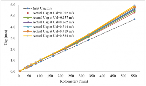
(b) Actual Usg at 30-degree pipe angle
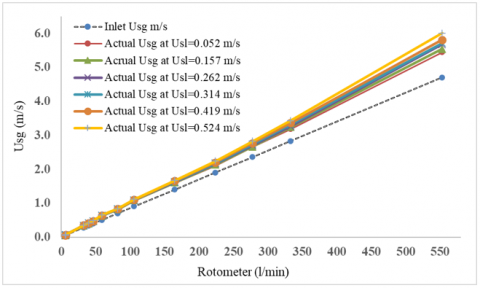
(c) Actual Usg at 45-degree pipe angle
Figure 2. The correlations of Usg rates at constant Usl changed from 0.052 to 0.524 m/s od different pipe rotation angles 0, 30, and 35 degrees
The effect of system pressure can influence the results; thus, pressure was measured simultaneously using a gauge pressure type (BUDENBERG, 0-15 lb/in2) to correlate the actual gas superficial velocities. The actual gas velocities were estimated from the calculations of Equations 4 and 5 at the different pipe orientations are illustrated in Figure 2.
Moreover, a calibration has made between the readings of the differential pressure transducer and the outlet voltages to derive the relationship between them as showed in Figure 3.
Figure 3. The calibration of the differential pressure cell with the outlet volts
The recorded pressure gradients by the Differential Pressure Transducer (DPT) and the flow patterns of oil-gas flow in a pipe of internal diameter 50 mm at different orientations 0, 30, and 45 degrees have been investigated and classified under various methods that conducted in many published studies such as in the researches [13, 27, 28]. The followed sections illustrate how the results have been analyzed.
3.1 Analysis of PDF with pressure gradient, and pressure gradient with time series
The value of pressure drops can identify the type of flow pattern created inside the pipe, as well as, pressure drops participated in the calculation of the flow energy of any transportation system. The current work investigates the relationship between the fluctuation of the pressure gradients in terms of time series, also the identification of flow patterns is conducted by analyzing the relationship between Probability Density Functions (PDF) with pressure losses. Figure 4, presents the pressure drop at Usl value of 0.052 m/s and Usg ranged from 0.05 to 0.062 m/s, the plot of PDF was recorded as the peak at PDF value of 1 at near-zero pressure gradient of all pipe orientations (0, 30, and 45-degrees). It was observed undetectable fluctuations in pressure gradients under the time, and the flow was stable. Regarding the low amounts of gas and oil in the flow lines of 0 and 30-degree orientation, the stratified flow is reasonable, it is led to the fact that there is no pressure drop fluctuation occurs when the two-phase flow as layers and stable. When the tested pipe increases more to 45-degree, the cross-sectional area of the pipe is gradually filled with oil affected by the gravity force, so bubbly flow is observed at the same moment under the low value of gas superficial velocity.
As demonstrated in Figure 5, the flow pattern in a pipe of 0-degree orientation is also not impacted by the increase of the value of Usg to 0.28 m/s, while the observed alteration in patterns was clearly in 30, and 45-degree pipe angles. The feature of the PDF plot showed more than one peak at a PDF value of 0.07 with a large base of pressure gradient ranged from 0 to 0.4, and the characterization of pressure gradients with time series are fluctuating at values ranging from 0 to 200 (Pa/cm). The stratified flow regime changed to stratified-wavy influenced by the increasing value of the gas superficial velocity. The two-phase flow pattern in the 45-degree pipe rotation tend to conduct as a slug flow, and the feature of this flow can be observed from the PDF cure as one peak 0.035 with pressure gradient drop valued from 0 to 0.5, also the recorded pressure losses fluctuated at pressure gradient value ranged from 0 to 300 (Pa/cm).
Figure 4. The plots of the pressure gradient of time series and the PDF of pressure gradients in a pipe of the orientation of 0, 30, and 45-degree at Usl 0.052 m/s
Figure 5. The plots of the pressure gradient of time series and the PDF of pressure gradients in a pipe of the orientation of 0, 30, and 45-degree at Usl 0.052 m/s
In spite, the increment of Usg value reached 0.34 m/s, this did not affect the flow pattern in the 0-degree pipe position. However, this increase waved the flow mixture in 30-degree pip to produce a slug flow pattern, the plot of PDF showed one peak at PDF value 0.04 with based pressure gradient ranged from 0 to 0.5. Pressure gradients fluctuated between 0 and 350 (Pa/cm) as shown in Figure 6. Furthermore, at the Usg value of 0.34 m/s in the 30-degree pipe orientation, slug flow was characterized by many peaks at a mean PDF value of 0.04 with a pressure gradient base ranged from 0 to 0.6, and pressure losses oscillated between 0 and 300 (Pa/cm). The regimes of two-phase flow remained unchanged in the different tested pipe orientations, even when the value of Usg reached near 5 m/s.
Figure 6. The plots of the pressure gradient of time series and the PDF of pressure gradients in a pipe of the orientation of 0, 30, and 45-degree at Usl 0.052 m/s
The flow regimes were identified at Usl value of 0.157 m/s in the examined pipe orientation at the various stages of Usg rates are very similar to those flow patterns were indicated at Usl value of 0.052 m/s.
The flow patterns were observed at the constant value of Usl 0.262 m/s and ranged values of Usg 0.05 and 0.062 m/s are stratified flow in the horizontal flow line, stratified and slug flow pattern in the pipe of a 30-degree angle, and bubbly flow in the pipe of 45-degree. By increasing the value of Usg progressively, stratified flow in the horizontal pipe unchanged at Usg ranged from 0.28 to 0.4 m/s, the wavy flow was observed at Usg rated from 0.34 to 0.4 m/s in the 30-degree pipe orientation, and slug flow was noticed at Usg varied from 0.34 to 0.5 m/s in the 45-degree pipe rotation. The stratified flow pattern was also identified at every rate of Usg in the 0-degree pipe angle, while slug flow was indicated at Usg 0.5 m/s comparing with the wavy flow pattern that occurred in the lower values of Usg rates, besides, the slug flow is observed as well in the 45-degree pipe at Usg 0.5 m/s as illustrated in Figure 7.
Figure 7. The plots of the pressure gradient of time series and the PDF of pressure gradients in a pipe of the orientation of 0, 30, and 45-degree at Usl 0.262 m/s
The increasing values of Usl are significantly affecting the flow types especially those that flow near to the horizontal flow line because of the impact of gravity. When the values of Usg are near 5 m/s and pipe orientation of 45-degree as demonstrated in Figure 8.
Figure 8. The plots of the pressure gradient of time series and the PDF of pressure gradients in a pipe of the orientation of 0, 30, and 45-degree at Usl 0.262 m/s
As explained by Hernandez-Perez [29], when the amount of liquid is increased in the horizontal pipe, stratified flow altered to bubbly flow (Figure 8.a), the only disadvantage of using the DPT as a sensor for detecting the flow patterns, the behavior of the pressure gradients is similar in both mentioned flow patterns.
The plot of PDF in the 45-degree pipe angle showed one peak at 0.035 with a large base of pressure drop indicated from 0 to 0.8. The two plots denote the churn flow.
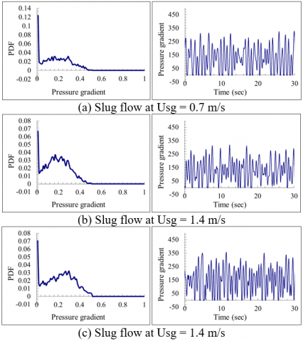
The flow regimes were indicated in the all-tested conditions at Usl values of 0.314, 0.419 and 0.524 m/s are very similar to those flow regimes which are observed at Usl 0.262 m/s except that, the slug flow is observed lately in the 30-degree flow lines orientation where it is estimated at Usg values ranged from 0.7 to 1.4 m/s at Usl values 0.314, 0.419 and 0.524 m/s respectively as shown in Figure 9.
Figure 9. The plots of the pressure gradient of time series and the PDF of pressure gradients in a pipe of the orientation 30-degree at Usl values; (a) 0.314 m/s, (b) 0.419 m/s, and (c) 0.524 m/s
3.2 Total pressure drops with mean void fractions
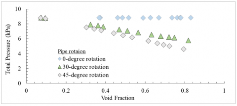
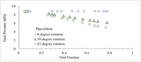
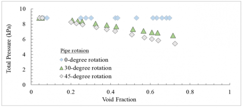
As demonstrated in Figure 10, the relationships between the total pressure drops (kPa) with the void fractions that recorded by ECT, generally, total pressure drops diminished with increasing the amount of gas flow rate and the drops increased with increment the value of liquid flow rate. At any constant value of Usl under the test conditions, total pressure gradients declined sharply to down with levering the pipe’s angle from 0-degree to 45-degree component with boosting the amount of void fraction. Raising the angle level of the tested pipe led to increasing gravity force and then raising total pressure drops inside the pipe but the little amount of liquid also makes flow lighter, as a result, decreasing total pressure drops.
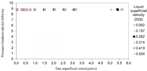
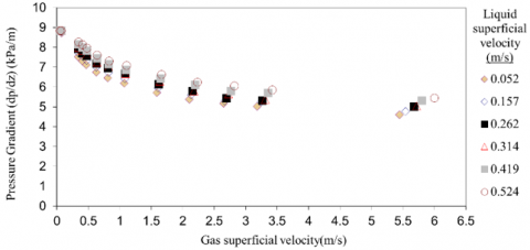
3.3 Pressure gradients vs gas superficial velocities (Usg)
The analysis of pressure gradients (dp/dz) with the superficial velocities of gas was performed for 0, 30, and 45-degree pipe orientation at different superficial velocities of both phases. As shown in Figure 11 (a) in 0-degree pipe orientation, pressure gradients (dp/dz) increased with worthless values by increasing the flow rate of gas and it was recorded about 8.80 kPa/m for all values of Usl rates.
(a) At the liquid superficial velocity of 0.052 m/s
(b) At the liquid superficial velocity of 0.262 m/s
(c) At the liquid superficial velocity of 0.524 m/s
Figure 10. Total pressure gradient (kPa) with void fractions at the pipe of orientations 0, 30, and 45-degrees
(a) dp/dz vs Usl rates at 0-degree pipe rotation
(b) dp/dz vs Usl rates at 30-degree pipe rotation
(c) dp/dz vs Usl rates at 45-degree pipe rotation
Figure 11. Pressure gradient (dp/dz), kPa with Usg rates at constant values of Usl in a pipe of orientations 0, 30, and 45-degrees
The behavior of the plot was conducted near the straight line because of the influence of the frictional drop affected only. Gravitational pressure drops in a horizontal pipe are equal in a one-meter pipe length (dz) with assuming the flow is near to homogenous. As Figure 10 (b and c) showed, gravitational pressure drops increased when the pipe was filled with liquid, thus (dp/dz) decreased with adding more amount of gas flow rates to the flow. Accordingly, at the constant value of Usl rates, pressure gradients rose by increasing the pipe’s angle, furthermore, the total pressure gradient rises when the gravitational pressure gradient increases. The main pressure gradient also affected by the frictional pressure drop as a result of adding more amount of liquid in the pipe, and it contributes to the increasing total pressure gradients.
Using gradient pressure analysis is very useful to identify the flow patterns of two-phase oil-gas flow that occurred inside near to horizontal flow lines in pipes. Tomographic sensors like WMS or ECT are considered to be very accurate devices for such tasks but with an expensive initial value of cost. The Differential Pressure Transducer that is used in the current study was beneficial with a low-cost value device to estimate the flow patterns of the two-phase flow in inclined pipes.
The analysis of the Probability Density Function (PDF) of the pressure gradient and the relationship between the pressure gradient and time series revealed that; the stratified flow pattern is observed in the 0-degree pipe orientation at lower and moderate flow rates. The flow pattern in the indicated pipe of 30 and 45-degree is altered by increasing the values of superficial velocities and because of the effect of gravitational and bouncy forces. At the different Usl values of the 30-degree pipe orientation; the stratified flow pattern is observed at low values of Usg, wavy flow is indicated at moderate values of Usg, and the slug flow pattern is classified at higher values of Usg. At the various Usl values of 45-degree pipe angle; slug flow has been observed as a dominant flow pattern in most values of Usg, whereas churn flow pattern is classified at higher values of Usg (near to 5 m/s).
This study is financed by the Research Center of Multiphase Flow - College of Engineering at University of Zakho. The authors would like to express their deep gratitude to the people in charge of this center “This work was supported by the Scientific Research Ministry of Iraqi Kurdistan Region-University of Zakho-College of Engineering as a part of the multiphase flow Research Center under Grant number 9870’’.
|
g |
gravitational acceleration, m.s-2 |
|
$\mathrm{U}_{\mathrm{sl}}$ $\mathrm{U}_{\mathrm{sg}}$ |
the superficial velocity of liquid, m.s-1 the superficial velocity of gas, m.s-1 |
|
Re D |
Reynold number diameter, m |
|
h |
static head, m |
|
v |
velocity, m.s-1 |
|
Ap |
pipe cross-section area, m2 |
|
Q |
volume flowrate, m3.s-1 |
|
$\frac{d p}{d z}$ |
total gradient pressure drops, Pa |
|
$\left(\frac{d p}{d z}\right)_{f r i c}$ |
frictional pressure drops, Pa |
|
$\left(\frac{d p}{d z}\right)_{\operatorname{grav}}$ |
gravitational pressure drops, Pa |
|
$\left(\frac{d p}{d z}\right)_{a c c e}$ |
acceleration pressure drops, pa |
|
Greek symbols |
|
|
a |
void fraction |
|
σ |
surface tension. N.m-1 |
|
$\rho_{\text {liq }}$ |
liquid density, kg.m-3 |
|
$\rho_{\text {gas }}$ |
gas density, kg.m-3 |
|
∆p |
differential pressure, Pa |
|
$\mathrm{C}_{\mathrm{f}}$ |
Friction factor |
|
$\rho_{\mathrm{A}}$ |
gas density at the variable area, kg. m-3 |
|
$\rho_{\mathrm{R}}$ |
the reference gas density, kg. m-3 |
|
Subscripts |
|
|
PSD |
Power Spectral Density |
|
|
Probability Density Function |
|
ECT |
Electrical Capacitance Tomography |
|
WMS |
Wire Mesh sensor |
|
DPT |
Differential Pressure Transducer |
[1] Abdulkareem, L.A., Escrig, E., Reinecke, S., Hewakandamby, B.N., Azzopardi, B.J. (2016). Tomographic interrogation of gas-liquid flows in inclined risers. In ICMF-2016–9th International Conference on Multiphase Flow, Firenze, Italy.
[2] Berger, S.A., Talbot, L., Yao, L.S. (1983). Flow in curved pipes. Annual Review of Fluid Mechanics, 15(1): 461-512. https://doi.org/10.1248/cpb.37.3229
[3] Abdulkadir, M., Zhao, D., Sharaf, S., Abdulkareem, L., Lowndes, I.S., Azzopardi, B.J. (2011). Interrogating the effect of 90° bends on air–silicone oil flows using advanced instrumentation. Chemical Engineering Science, 66(11): 2453-2467. https://doi.org/10.1016/j.ces.2011.03.006
[4] Lin, Z., Liu, X., Lao, L., Liu, H. (2020). Prediction of two-phase flow patterns in upward inclined pipes via deep learning. Energy, 210: 118541. https://doi.org/10.1016/j.energy.2020.118541
[5] Brauner, N., Maron, D.M. (1992). Flow pattern transitions in two-phase liquid-liquid flow in horizontal tubes. International Journal of Multiphase Flow, 18(1): 123-140. https://doi.org/10.1016/0301-9322(92)90010-E
[6] Angeli, P., Hewitt, G.F. (1999). Pressure gradient in horizontal liquid–liquid flows. International Journal of Multiphase Flow, 24(7): 1183-1203. https://doi.org/10.1016/S0301-9322(98)00006-8
[7] Brinkman, H.C. (1952). The viscosity of concentrated suspensions and solutions. The Journal of Chemical Physics, 20(4): 571-571. https://doi.org/10.1063/1.1700493
[8] Picchi, D., Strazza, D., Demori, M., Ferrari, V., Poesio, P. (2015). An experimental investigation and two-fluid model validation for dilute viscous oil in water dispersed pipe flow. Experimental Thermal and Fluid Science, 60: 28-34. https://doi.org/10.1016/j.expthermflusci.2014.07.016.
[9] Hubbard, M.G. (1966). The characterization of flow regimes for horizontal two-phase flow. Proc. Heat Transf. Fluid Mech. Inst., 1966: 100-121.
[10] Jones Jr, O.C., Zuber, N. (1975). The interrelation between void fraction fluctuations and flow patterns in two-phase flow. International Journal of Multiphase Flow, 2(3): 273-306. https://doi.org/10.1016/0301-9322(75)90015-4
[11] Taitel, Y., Bornea, D., Dukler, A.E. (1980). Modelling flow pattern transitions for steady upward gas-liquid flow in vertical tubes. AIChE Journal, 26(3): 345-354. https://doi.org/10.1002/aic.690260304
[12] Perez, V.H. (2007). Gas-liquid two-phase flow in inclined pipes. Notthinghan: [sn].
[13] Abdulkareem, L.A., Azzopardi, B.J., Hunt, A. (2011). Tomographic investigation of gas-oil flow in inclined risers. Doctoral dissertation, University of Nottingham. https://doi.org/10.1115/AJTEC2011-44546
[14] Jia, J., Babatunde, A., Wang, M. (2015). Void fraction measurement of gas–liquid two-phase flow from differential pressure. Flow Measurement and Instrumentation, 41: 75-80. https://doi.org/10.1016/j.flowmeasinst.2014.10.010
[15] De Salve, M., Monni, G., Panella, B. (2012). Horizontal air-water flow analysis with wire mesh sensor. In Journal of Physics: Conference Series, 395(1): 012179. https://doi.org/10.1088/1742-6596/395/1/012179
[16] Hanafizadeh, P., Hojati, A., Karimi, A. (2015). Experimental investigation of oil–water two phase flow regime in an inclined pipe. Journal of Petroleum Science and Engineering, 136: 12-22. https://doi.org/10.1016/j.petrol.2015.10.031
[17] Yao, C., Li, H., Xue, Y., Liu, X., Hao, C. (2018). Investigation on the frictional pressure drop of gas liquid two-phase flows in vertical downward tubes. International Communications in Heat and Mass Transfer, 91: 138-149. https://doi.org/10.1016/j.icheatmasstransfer.2017.11.015
[18] Musa, V.A., Abdulkareem, L.A., Ali, O.M. (2019). Experimental study of the two-phase flow patterns of air-water mixture at vertical bend inlet and outlet. Engineering, Technology & Applied Science Research, 9(5): 4649-4653. https://doi.org/10.48084/etasr.3022
[19] Wen, Y., Wu, Z., Wang, J., Wu, J., Yin, Q., Luo, W. (2017). Experimental study of liquid holdup of liquid-gas two-phase flow in horizontal and inclined pipes. International Journal of Heat and Technology, 35(4): 713-720. https://doi.org/10.18280/ijht.350404
[20] Garcia, F., García, R., Joseph, D.D. (2005). Composite power law holdup correlations in horizontal pipes. International Journal of Multiphase Flow, 31(12): 1276-1303. https://doi.org/10.1016/j.ijmultiphaseflow.2005.07.007
[21] Vohra, I.R., Hernandez, F., Marcano, N., Brill, J.P. (1975). Comparison of liquid-holdup and friction-factor correlations for gas-liquid flow. Journal of Petroleum Technology, 27(5): 564-568. https://doi.org/10.2118/4690-PA
[22] Baghernejad, Y., Hajidavalloo, E., Zadeh, S.M.H., Behbahani-Nejad, M. (2019). Effect of pipe rotation on flow pattern and pressure drop of horizontal two-phase flow. International Journal of Multiphase Flow, 111: 101-111. https://doi.org/10.1016/j.ijmultiphaseflow.2018.11.012
[23] Da Silva, M.J., Thiele, S., Abdulkareem, L., Azzopardi, B.J., Hampel, U. (2010). High-resolution gas–oil two-phase flow visualization with a capacitance wire-mesh sensor. Flow Measurement and Instrumentation, 21(3): 191-197. https://doi.org/10.1016/j.flowmeasinst.2009.12.003
[24] Abdulkareem, L.A., Musa, V.A., Mahmood, R.A., Hasso, E.A. (2021). Experimental investigation of two-phase flow patterns in a vertical to horizontal bend pipe using wire-mesh sensor. Revista de Chimie, 71(12): 18-33. https://doi.org/10.37358/rc.20.12.8383
[25] Hampel, U., Speck, M., Koch, D., Menz, H.J., Mayer, H.G., Fietz, J. (2005). Experimental ultra fast X-ray computed tomography with a linearly scanned electron beam source. Flow Measurement and Instrumentation, 16(2-3): 65-72. https://doi.org/10.1016/j.flowmeasinst.2005.02.002
[26] Zhu, K., Rao, S.M., Wang, C.H., Sundaresan, S. (2003). Electrical capacitance tomography measurements on vertical and inclined pneumatic conveying of granular solids. Chemical Engineering Science, 58(18): 4225-4245. https://doi.org/10.1016/S0009-2509(03)00306-3
[27] Abdulkadir, M., Jatto, D.G., Abdulkareem, L.A., Zhao, D. (2020). Pressure drop, void fraction and flow pattern of vertical air–silicone oil flows using differential pressure transducer and advanced instrumentation. Chemical Engineering Research and Design, 159: 262-277. https://doi.org/10.1016/j.cherd.2020.04.009
[28] Abdulkadir, M. (2011). Experimental and computational fluid dynamics (CFD) studies of gas-liquid flow in bends. Doctoral dissertation, University of Nottingham.
[29] Hernandez-Perez, V. (2008). Gas-liquid two-phase flow in inclined pipes. PhD thesis, University of Nottingham.