Ahmed Bensenouci* | Mohamed Teggar | Ahmed Medjelled | Ahmed Benchatti
© 2021 IIETA. This article is published by IIETA and is licensed under the CC BY 4.0 license (http://creativecommons.org/licenses/by/4.0/).
OPEN ACCESS
Most thermochemical cycles require complex thermal processes at very high temperatures, which restrict the production and the use of hydrogen on a large scale. Recently, thermochemical cycles producing hydrogen at relatively low temperatures have been developed in order to be competitive with other kinds of energies, especially those of fossil origin. The low temperatures required by those cycles allow them to work with heats recovered by thermal, nuclear and solar power plants. In this work, a new thermochemical cycle is proposed. This cycle uses the chemical elements Magnesium-Chlorine (Mg-Cl) to dissociate the water molecule. The configuration consists of three chemical reactions or three physical steps and uses mainly thermal energy to achieve its objectives. The highest temperature of the process is that of the production of hydrochloric acid, HCl, estimated between 350-450℃. A thermodynamic analysis was performed according to the first and second laws by using Engineering Equation Solver (EES) software and the efficiency of the proposed cycle was found to be 12.7%. In order to improve the efficiency of this cycle and make it more competitive, an electro-thermochemical version should be studied.
exergy analysis, hydrogen production, magnesium-chlorine cycle, thermochemical cycle, water splitting
The rapid rising world energy demand and climate change due to greenhouse gas emissions, have motivated the public and private sectors, to seek an alternative to conventional energies and limited ecological damage. The solution to those problems is the use of renewable energies. Currently, the world consumes about 85 million barrels of oil and 2.94 billion cubic meters of natural gas a day [1], releasing greenhouse effect gases that cause global warming. Unlike fossil fuels, hydrogen is a clean and sustainable energy carrier, which is widely considered the fuel of the next generation. The production of hydrogen from the dissociation of water molecule constitutes an interesting process of energy production which has the potential to be sustainable development. Hydrogen demand is expected to increase significantly over the next decades. The hydrogen market worldwide is currently growing by 10% per year, reaching between 20 and 40% by the year 2020 [2]. The prevailing process for hydrogen production at large scale is the steam-reforming of methane. This technology emits huge amounts of carbon dioxide as the primary greenhouse effect gas. On the other hand, the production of hydrogen based on thermochemical cycles does not emit harmful gases. The thermal energy required for the operation of these systems can be supplied in abundance for large-scale capacities either by heat recovered from thermal and nuclear power plants or directly by solar power plant [3, 4]. The thermochemical cycles of hydrogen production have received more attention because current estimates indicate that the production costs of H2 by these methods could be as low as 60% of those from room temperature electrolysis [5, 6]. Thermochemical cycles are more profitable than electrolysis on the hydrogen generation as they avoid the intermediate process of generating electricity before hydrogen is produced. Since the beginning of the development of thermochemical cycles four decades ago, a very long list of 280 thermochemical cycles [7] of water decomposition has been discovered, but few of them have undergone exhaustive studies and have promising results. Hydrogen can be produced using fossil fuels, water and biomass [8]. Water is one of the most promising resources for hydrogen production because of its abundance and equitable accessibility on the globe as well as its price which is almost symbolic compared to other sources of energy. Water can be broken down into hydrogen and oxygen by several technologies. High and low temperature electrolysis, photochemical and radiochemical systems, pure and hybrid thermochemical separation cycles are prospective technologies for hydrogen production.
Several types of thermochemical processes exist for the production of hydrogen. The sulfur-iodine-based cycle (S-I) was proposed by General Atomics of the United States of America in the mid-1970s. These are the three chemical reactions that produce the dissociation of water molecule, the highest temperature of the cycle is estimated at 850℃. This cycle has a thermal efficiency of approximately 47% and potentially reaches 60% efficiency with cogeneration of hydrogen and electricity [9, 10]. The UT-3 cycle is a thermochemical cycle of hydrogen production initially developed at the University of Tokyo. This cycle is based essentially on the chemical elements which are bromine, calcium and iron (Br-Ca-Fe). The cycle consists of four steps that include only solid and gaseous components, the maximum temperature is about 750℃. The predicted thermal efficiency of the UT-3 cycle varies between 35-50%, depending on the efficiency of the membrane separators, and whether the electricity is co-generated with hydrogen or not [11-13]. Copper-chlorine (Cu- Cl) is identified as a promising cycle for thermochemical hydrogen production by Atomic Energy of Canada Limited (AECL) [14, 15]. Water is decomposed into hydrogen and oxygen via copper and chlorine compounds. This cycle is intended to operate at a temperature of 550℃. The energy efficiency of the process should be around 40-45% [16, 17]. Recently, it has been upgraded to 47.4% performance in the US Argonne National Laboratory (ANL) [18, 19]. In this work, a thorough thermodynamic study of the Magnesium – chlorine (Mg-Cl) cycle is performed (Figure 1). The study was conducted with the aid of exergy analysis which allows analyzing thermodynamic systems from effective view point. Various evaluations are carried out using several analyzes and tools of thermodynamics and thermochemistry [20, 21]. The three chemical reactions of the proposed system are newly introduced to a thermochemical cycle and validated with simulations and previous studies. The simulations and the thermodynamic modeling of the results were performed with the Engineering Equation Solver (EES) software [22]. This work focuses on the details of the proposed Mg-Cl cycle to identify strengths, weaknesses and gaps by developing new methods for more efficient and cos t-effective hydrogen production.
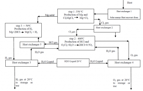
Figure 1. Process flow diagram of the proposed Mg-Cl cycle
The proposed thermochemical cycle based on magnesium and chlorine consisting of three main steps, is summarized in Table 1. The main chemical reaction is the reaction of hydrogen production while the other reactions are for the recycling of the chemical elements for the continuity of the operation of the cycle. The process is first described by a decomposition transformation of solid magnesium chloride at the highest cycle temperature of 350-450℃ to produce magnesium in the solid phase and chlorine gas. The second step is the reaction of chlorine gas and liquid water or vapor to produce two moles of HCl and one-half mole of oxygen gas. This reaction is called the inverse Deacon reaction. Mg and HCl react in the last step to form one mole of MgCl and two moles of hydrogen H2. These chemical reactions form an internal recycling loop of elements and components in continuous form.
Table 1. Steps and reactions of the proposed cycle
|
Stage |
Reaction |
Temperature °C / Pressureatm |
|
1. Mg and Cl2 Production |
MgCl2(s)+ Q →Mg(s)+Cl2(g) |
300°C-400°C/ 1atm |
|
2. HCl and O2 Production |
Cl2 (g) +H2O(l/g)+ Q→2HCl(g)+1/2O2(g) |
350-450°C/1atm |
|
3. H2 Production |
Mg(s)+2HCl(g) →MgCl2(s)+H2(g)+Q |
<50°C/1atm |
|
Q: Heat; g: gas; l: liquid; s: solid |
||
The realization of thermochemical conversion depends on each reaction in the steps of the cycle. Therefore, it can be examined with the Gibbs function whether these reactions will occur. The variation of Gibbs free energy (ΔG) at constant temperature is defined by:
ΔG = ΔH - T ΔS < 0 (1)
G: Gibbs function, is a function of state.
The previous derivation shows that at constant temperature and pressure:
- if ΔG <0: the reaction is feasible and spontaneous
- if ΔG> 0: the reaction is not feasible and non-spontaneous (the reaction is spontaneous in the opposite direction)
- if ΔG = 0: the system is in equilibrium
The reactions tested are:
MgCl2(s)+ Q →→Mg(s)+Cl2(g) (2)
Cl2 (g) +H2O(l/g)+ Q→2HCl(g)+1/2O2(g) (3)
Mg(s)+2HCl(g) +Q→MgCl2(s)+H2(g) (4)
The Figures 2, 3 and 4 illustrate that all steps are feasible because of their Gibbs’s functions are less than zero, it can be said that the function of Gibbs increases in the negative sense with the increase of the temperature that means that these reactions will be more spontaneous and more profitable in the temperature ranges which correspond to ΔG high in absolute value.
Figure 2. Variation of ΔG as a function of the reaction temperature for the first step
Figure 3. Variation of ΔG as a function of the reaction temperature for the second step
Figure 4. Variation of ΔG as a function of the reaction temperature for the third step
According to the principle of the conservation of the mass for a system under a steady state the mass in term of flow remains constant at the entry and the exit [23-25];
$\sum_{i n} \dot{m}=\sum_{o u t} \dot{m}$ (5)
4.1 The first law analysis
For an open steady-state system the variation of the total energy is zero,
$\dot{E}_{i n}-\dot{E}_{o u t}=\frac{d E_{s y s}}{d t}=0$ (6)
Energy can be conserved;
$\dot{E}_{i n}=\dot{E}_{\text {out }}$ (7)
For an open system, the first law of thermodynamics is written as follows;
$\begin{aligned} \dot{Q}-\dot{W}=\sum_{i n} \dot{m}(& \left.h+\frac{\theta^{2}}{2}+g z\right) \\ &-\sum_{o u t} \dot{m}\left(h+\frac{\theta^{2}}{2}+g z\right) \end{aligned}$ (8)
For a chemical process system, the specific enthalpy must be expressed relative to the standard conditions,
$\bar{h}=\overline{h_{f}^{\circ}}+\left(\bar{h}-\bar{h}^{\circ}\right)$ (9)
$\begin{aligned} \dot{Q}-\dot{W}=\sum_{i n} \dot{m}(& \left.\overline{h_{f}^{\circ}}+\left(\bar{h}-\bar{h}^{\circ}\right)+\frac{\theta^{2}}{2}+g z\right) \\ &-\sum_{o u t} \dot{m}\left(\overline{h_{f}^{\circ}}+\left(\bar{h}-\bar{h}^{\circ}\right)+\frac{\theta^{2}}{2}\right.\\ &+g z) \end{aligned}$ (10)
Since the number of moles differs between the reactants and the products of the reaction:
$\begin{aligned} \dot{Q}-\dot{W}=\sum_{i n} \dot{m} \cdot N_{r} &\left(\overline{h_{f}^{\circ}}+\left(\bar{h}-\bar{h}^{\circ}\right)+\frac{\theta^{2}}{2}+g z\right) \\ &-\sum_{o u t} \dot{m} \cdot N_{p}\left(\overline{h_{f}^{\circ}}+\left(\bar{h}-\bar{h}^{\circ}\right)+\frac{\theta^{2}}{2}\right.\\ &+g z) \end{aligned}$ (11)
Mechanical work, kinetic and potential energy are zero W=Ec=EP=0.
Mass flow is assumed equal to unity,
$\dot{Q}=\sum_{i n} N_{r}\left(\overline{h_{f}^{\circ}}+\left(\bar{h}-\bar{h}^{\circ}\right)\right)_{r}-\sum_{o u t} N_{p}\left(\overline{h_{f}^{\circ}}+\left(\bar{h}-\bar{h}^{\circ}\right)\right)_{p}$ (12)
4.2 The second law analysis
The variation of the exergy of an open system is written as:
$\Delta E x=\left(H_{2}-H_{1}\right)-T_{0}\left(S_{2}-S_{1}\right)+m \frac{\Theta_{2}^{2}-\theta_{1}^{2}}{2}$
$+m g\left(z_{2}-z_{1}\right)$ (13)
The molar specific exergy of an open system is written:
$\Delta e x=\left(\overline{h_{2}}-\overline{h_{1}}\right)-T_{0}\left(\overline{s_{2}}-\overline{s_{1}}\right)+\frac{\theta_{2}^{2}-\theta_{1}^{2}}{2}+g\left(z_{2}\right.$
$\left.-z_{1}\right)$ (14)
The destroyed exergy is proportional to the entropy generation caused by the irreversibilities related with the process [26, 27]:
$E x_{d e t}=T_{0} S_{g e n} \geq 0$ (15)
For an open system, undergoing chemical interactions:
$\begin{aligned} \sum\left(1-\frac{T_{0}}{T}\right) Q-(W&-P_{0}\left(V_{2}-V_{1}\right)+\sum_{i n} m \cdot E x \\ &-\sum_{o u t} m . E x-T_{0} S_{g e n}+E x^{c h m} \\ &=E x_{2}-E x_{1} \end{aligned}$ (16)
After simplification, the following equation is obtained:
$\sum\left(1-\frac{T_{0}}{T}\right) Q+\sum_{i n} m E x-\sum_{o u t} m E x-T_{0} S_{g e n}+E x^{c h m}=0$ (17)
We are interested in the performance of chemical reactions. We will calculate the rate of exergy destruction. The exergy destruction per unit of mole is therefore written:
$\overline{E x}_{d e t}=\sum_{i n}\left(\left(\bar{h}-\bar{h}_{0}\right)-T_{0}\left(\bar{s}-\overline{s_{0}}\right)+\overline{E x}^{c h m}\right)$
$-\sum_{o u t}\left(\left(\bar{h}-\bar{h}_{0}\right)-T_{0}\left(\bar{s}-\bar{s}_{0}\right)\right.$
$\left.+\overline{E x}^{c h m}\right)+\sum\left(1-\frac{T_{0}}{T_{\text {reaction }}}\right) Q$ (18)
$\overline{E x}^{c h m}=-\Delta G+\sum_{P} N \cdot \overline{E x}^{c h m}-\sum_{R} N \cdot \overline{E x}^{c h m}$ (19)
The function of Gibbs, is written as:
$d G=H-T d S \leq 0$ (20)
The function of Gibbs is always negative or equal to zero. Thus, the chemical reactions at the specified temperature and pressure always proceed in the decreasing direction of the Gibbs function, since otherwise the second principle of thermodynamics will not be respected [28].
The enthalpy and mass entropy of each compound of the chemical reaction are evaluated as follows:
$d h=\int_{T_{0}}^{T_{\text {reac }}} C_{p}(T) \cdot d T$ (21)
$d s=\int_{T_{0}}^{T_{r e a c}} C_{p}(T) \cdot \frac{d T}{T}-R \cdot \ln \frac{P_{r e a c}}{P_{0}}$ (22)
The heat capacity, the specific enthalpy and entropy are expressed as a function of the temperature and several coefficients, Table 2. Among all the polynomial developments proposed in the literatures, the most used and the most precise ones are the Shomate equations [29].
$c_{p, i}=A_{i}+B_{i} . t+C_{i} . t^{2}+D_{i} . t^{3}+\frac{E_{i}}{t^{2}}$ (23)
$\begin{aligned} \bar{h}_{t, i}-\bar{h}_{0, i}=A_{i} . t &+B_{i} \cdot \frac{t^{2}}{2}+C_{i} \cdot \frac{t^{3}}{3}+D_{i} \cdot \frac{t^{4}}{4}-E_{i} \cdot \frac{1}{t} \\ &+F_{i}-H_{i} \end{aligned}$ (24)
$\begin{aligned} \bar{s}_{t, i}=A_{i} \cdot \ln (t)+& B_{i} \cdot t+C_{i} \cdot \frac{t^{2}}{2}+D_{i} \cdot \frac{t^{3}}{3}-E_{i} \cdot \frac{1}{2 t^{2}} \\ &+G_{i}-R \cdot \ln \frac{P_{r e a c}}{P_{0}} \end{aligned}$ (25)
$t=\frac{T}{1000}$ (26)
4.3 First step analysis
MgCl2 is introduced into a reactor where its temperature is raised to 250 to 350℃, the process is assumed to be steady state and adiabatic. In this step, Eq. (2), the dissociation of MgCl2 is an endothermic chemical reaction.
The heat involved for this reaction is:
$Q=\left[N\left(\bar{h}_{f}^{\circ}+\bar{h}-\bar{h}^{\circ}\right)\right]_{M g}+\left[N\left(\bar{h}_{f}^{\circ}+\bar{h}-\bar{h}^{\circ}\right)\right]_{C l_{2}}$
$-\left[N\left(\bar{h}_{f}^{\circ}+\bar{h}-\bar{h}^{\circ}\right)\right]_{M g C l_{2}}$ (27)
The destroyed exergy can be written:
$\begin{aligned} \overline{E x}_{\text {dest }}=N_{M g C l_{2}} &\left[\left(\bar{h}-\bar{h}^{\circ}\right)-T_{0}\left(\bar{s}-\bar{s}^{\circ}\right)\right.\\ & \left.+\overline{E x}^{c h m}\right]_{M g C l_{2}} \\ &-N_{M g}\left[\left(\bar{h}-\bar{h}^{\circ}\right)-T_{0}\left(\bar{s}-\bar{s}^{\circ}\right)\right.\\ & \left.+\overline{E x}^{c h m}\right]_{M g} \\ &-N_{C l_{2}}\left[\left(\bar{h}-\bar{h}^{\circ}\right)-T_{0}\left(\bar{s}-\bar{s}^{\circ}\right)\right.\\ & \left.+E x^{c h m}\right]_{C l_{2}}+\left(1-\frac{T_{0}}{T_{\text {reac }}}\right) Q \end{aligned}$ (28)
Table 2. Different Shomate coefficients for different compounds [29]
|
compounds |
Shomate coefficients |
|||||||
|
A |
B |
C |
D |
E |
F |
G |
H |
|
|
H2(g) |
33,0661 |
-11,3634 |
11,432816 |
-2,772874 |
-0,158558 |
-9,980797 |
172,7079 |
0 |
|
Mg (s) |
26,54083 |
-1,533048 |
8,062443 |
0,57217 |
-0,174221 |
-8,501596 |
63,90181 |
0 |
|
HCl(g) |
32,12392 |
-13,458 |
19,86852 |
-6,853936 |
-0,049672 |
-101,6206 |
228,6866 |
-92,31201 |
|
MgCl2(s) |
78,30733 |
2,435888 |
6,858873 |
-1,728967 |
-0,729911 |
-667,5823 |
179,2693 |
-641,6164 |
|
Cl2(g) |
33,0506 |
12,2294 |
-12,0651 |
4,38533 |
-0,159494 |
-10,8348 |
259,029 |
0 |
|
H2O(g) |
30,092 |
6,832514 |
6,793435 |
-2,53448 |
0,082139 |
-250,881 |
223,3967 |
-241,8264 |
|
O2(g) |
29,659 |
6,137261 |
-1,186521 |
0,09578 |
-0,219663 |
-9,861391 |
237,948 |
0 |
4.4 Second stage analysis
The temperature range of this reaction changes from 450℃ to 500℃, Eq. (3). The temperature in this phase of the cycle is the highest. Thus the main requirement for this thermochemical cycle to operate is to have a thermal source whose temperature range is 450-500℃.
The heat involved in this reaction is:
$Q=\left[N\left(\bar{h}_{f}^{\circ}+\bar{h}-\bar{h}^{\circ}\right)\right]_{H C l}+\left[N\left(\bar{h}_{f}^{\circ}+\bar{h}-\bar{h}^{\circ}\right)\right]_{O_{2}}$
$-\left[N\left(\bar{h}_{f}^{\circ}+\bar{h}-\bar{h}^{\circ}\right)\right]_{c l_{2}}$
$-\left[N\left(\bar{h}_{f}^{\circ}+\bar{h}-\bar{h}^{\circ}\right)\right]_{H_{2} O}$ (29)
The exergy destruction is written as:
$\begin{aligned} \overline{E x}_{\text {dest }}=N_{C l_{2}}\left[\left(\bar{h}-\bar{h}^{\circ}\right)-T_{0}\left(\bar{S}-\bar{S}^{\circ}\right)+\overline{E x}^{c h m}\right]_{C l_{2}} \\+N_{H_{2} O}\left[\left(\bar{h}-\bar{h}^{\circ}\right)-T_{0}\left(\bar{s}-\bar{s}^{\circ}\right)\right. \left.+\overline{E x}^{c h m}\right]_{H_{2} O} \\-N_{H C l}\left[\left(\bar{h}-\bar{h}^{\circ}\right)-T_{0}\left(\bar{s}-\bar{s}^{\circ}\right)\right. \left.+\overline{E x}^{c h m}\right]_{H C l} \\ -N_{O_{2}}\left[\left(\bar{h}-\bar{h}^{\circ}\right)-T_{0}\left(\bar{s}-\bar{s}^{\circ}\right)\right. \left.+\overline{E x}^{c h m}\right]_{o_{2}}+\left(1-\frac{T_{0}}{T_{\text {xeac }}}\right) Q \end{aligned}$ (30)
4.5 Third stage analysis
The temperature required to carry out this reaction is less than 50℃, Eq. (4). This reaction is an adiabatic and endothermic transformation.
The heat involved in this reaction is:
$Q=\left[N\left(\bar{h}_{f}^{\circ}+\bar{h}-\bar{h}^{\circ}\right)\right]_{H_{2}}+\left[N\left(\bar{h}_{f}^{\circ}+\bar{h}-\bar{h}^{\circ}\right)\right]_{M g C l_{2}}$
$-\left[N\left(\bar{h}_{f}^{\circ}+\bar{h}-\bar{h}^{\circ}\right)\right]_{H C l}$
$+\left[N\left(\bar{h}_{f}^{\circ}+\bar{h}-\bar{h}^{\circ}\right)\right]_{M g}$ (31)
The destroyed exergy, is written as:
$\begin{aligned} \overline{E x}_{\text {dest }}=N_{M g}\left[\left(\bar{h}-\bar{h}^{\circ}\right)-T_{0}\left(\bar{s}-\bar{s}^{\circ}\right)+\overline{E x}^{c h m}\right]_{M g} +N_{H C l}\left[\left(\bar{h}-\bar{h}^{\circ}\right)-T_{0}\left(\bar{s}-\bar{s}^{\circ}\right)\right. \\ \left.+E x^{c h m}\right]_{H C l} -N_{M g c l_{2}}\left[\left(\bar{h}-\bar{h}^{\circ}\right)-T_{0}\left(\bar{s}-\bar{s}^{\circ}\right)\right. \left.+\overline{E x}^{c h m}\right]_{M g c l_{2}} -N_{H_{2}}\left[\left(\bar{h}-\bar{h}^{\circ}\right)-T_{0}\left(\bar{s}-\bar{s}^{\circ}\right)\right. \\ \left.+E x^{c h m}\right]_{H_{2}}+\left(1-\frac{T_{0}}{T_{\text {reac }}}\right) Q \end{aligned}$ (32)
To determine the molar heat and the destroyed exergy of the three chemical reactions, we need the values of specific standard enthalpies, entropies, chemical exergies and Gibbs functions of each of the molecules used in those reactions. The values of the previous functions for each compound are summarized in Tables 3 and Table 4.
Table 3. Enthalpy and standard entropy specific of chemical reaction compounds [30]
|
compounds |
Specific standard enthalpy of formation kJ/kmol |
Specific standard entropy kJ/kmol |
|
H2(g) |
0 |
130,6 |
|
Mg (s) |
0 |
32,67 |
|
HCl(g) |
-92310 |
186,9 |
|
MgCl2 |
-641620 |
89,62 |
|
Cl2 |
0 |
223,08 |
|
H2O(g) |
-241830 |
188,84 |
|
O2(g) |
0 |
205,07 |
Table 4. Gibbs function and standard chemical energy specific to chemical reaction compounds [30]
|
compounds |
Specific Gibbs function of formation kJ/kmol |
Specific standard chemical Exergy kJ/kmol |
|
H2(g) |
0 |
236090 |
|
Mg (s) |
0 |
629370 |
|
HCl(g) |
-95314 |
84531 |
|
MgCl2(s) |
-592113 |
160857 |
|
Cl2 |
0 |
123600 |
|
H2O(g) |
-228638 |
9437 |
|
O2(g) |
0 |
3970 |
4.6 Efficiency analysis
The exergy efficiency of the system can be evaluated as follows:
$\eta_{e x}=\frac{x_{\text {out }}}{x_{i n}}$ (33)
or
$\eta_{e x}=1-\frac{x_{\text {des }}}{x_{\text {in }}}$ (34)
The overall energy efficiency of the Mg-Cl cycle hydrogen production plant, can be expressed as the fraction of energy supplied by the useful energy based on the high heating value of hydrogen $\left(H H V_{H_{2}}\right)$, where $H H V_{H_{2}}=286030 k J / \mathrm{kmole}$ [30].
$\eta_{e n}=\frac{H H V_{H_{2}}}{Q_{\text {supp }}}$ (35)
5.1 Discussion and results of the first stage
Figure 5 shows the change of the amount of molar heat as a function of the variation of the temperatures of the reaction for the first stage [MgCl2(s) + Q → Mg(s) + 1/2Cl2(g)]. It can be seen, the molar heat produced is supplied to the system by the external medium. As the temperature of the reaction increases, the amount of the heat of reaction decreases. It is best to work at high temperatures in order to save the amount of heat supplied and therefore increase the cycle performance.
Figure 5. Variation of molar heat versus reaction temperature for the first stage
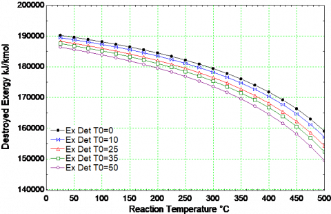
Figure 6. Change of exergy destruction versus the temperature reaction for several ambient temperature values
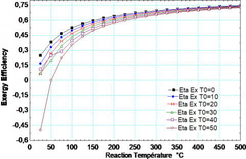
Figure 7. Change of the exergy efficiency as a function of the reaction temperature variation for different ambient temperatures values
In Figure 6, the destroyed exergy decreases in a non-linear way with the increase of the reaction temperature. Unlike energy, the value of the exergy depends at the same time on the state of the external environment as well as the state of the system. For this reason, the ambient temperature was varied. At Laghouat city, Algeria, ambient temperatures varies between 0℃ (in winter) and 50℃ (in summer).
The exergy efficiency of this stage, Figure 7, varies between 0.23 and 0.69. It increases with the elevation of the reaction temperature, because at high temperatures, the quality of the energy increases and consequently the exergy of the process will be better as irreversibilities decrease and this is the main cause of the improvement of the economic performance.
It can be seen that in the zone of low temperatures the yields are almost zero or sometimes even negative whereas their growth becomes very fast in the high temperatures.
5.2 Results and discussion of the second stage
Figure 8 shows the change of the molar heat versus the change of the temperatures of the reaction for the second stage [Cl2(g) + H2O (1/g) + Q → 2HCl(g)+1/2O2(g)]. Reaction temperatures vary in the range of 0℃ to 500℃. The chemical reaction is endothermic at this step. As the temperature of the reaction increases, the amount of the heat of reaction decreases. It is best to work at high temperatures in order to save the amount of heat supplied and therefore the performance cycle increase. The pace of the curve is almost linear.
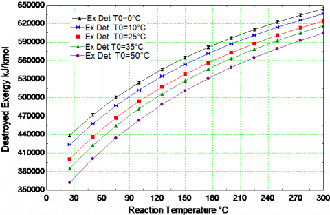
The exergy destruction decreases in a non-linear way with the increase of the reaction temperature for the different ambient temperatures (Figure 9). The curves of the destroyed exergy are in regression with the increase of the temperature. The exergy destruction rate decreased with the increase of the ambient temperature and the irreversibilities, such as heat transfer and chemical reactions. The irreversibilities within the thermodynamics system always causes entropy generation which lowers the quality and availability of energy.
The exergy efficiency of this stage, Figure 10, varies between 0.1 and 0.4, and it increases with the increase of the temperature of the reaction, because at high temperatures, the quality of the energy increases and consequently the exergy of the process will be better as irreversibilities decrease and this is the main cause of the improvement of the economic performance. It can be seen that in the zone of low temperatures the yields are almost zero whereas their growth becomes very fast in the high temperatures.
Figure 8. Variation of molar heat versus reaction temperature for the second stage
Figure 9. Change of destroyed exergy as a function of reaction temperature variation for several ambient temperatures
Figure 10. Change of the exergy efficiency versus the reaction temperature variation for different ambient temperatures
5.3 Results and discussion of the third stage
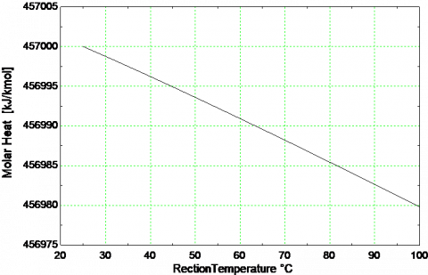
Figure 11 shows the change of the molar heat as a function of the variation of the temperatures of the chemical reaction produced during the process of the third step. Reaction temperatures vary in the range of 0℃ to 100℃. This temperature range is chosen because, by experience, all the corrosion reactions in which a metal and an acid are reacted are carried out at atmospheric pressure and at room temperature. In an experimental study carried out in our laboratories, various metals such as copper, zinc and magnesium were mixed with different acids, such as hydrochloric acid HCl and sulfuric acid H2SO4 for different concentrations, reacted completely and spontaneously at atmospheric pressure and at room temperature 24℃. The increase in temperature in this type of reaction up to 100℃ acts as a catalyst but the reaction efficiency does not increase so much. The chemical reaction [Mg(s) + 2HCl(g) → MgCl2(s) + H2(g) +Q] is exothermic in the third step. The product of this reaction is hydrogen.
It can be seen from Figure 11 that the amount of heat generated is rejected from the system to the outside environment. As the temperature of the reaction increases, the amount of the heat of reaction decreases very little. It can be assumed with a very good approximation that the value of the heat remains unchanged in the closed range of (0 - 100℃). It is better to work in this case at ambient temperatures (20-30℃) in order to save the amount of heat supplied and therefore increase the performance of the reaction as well as the entire cycle.
The exergy efficiency of this chemical reaction, Figure 13, varies between 0.62 and 0.96, for ambient temperatures of 0℃ and 50℃ respectively and for a reaction temperature close to 30℃ (ambient temperature). It is found that the performance at high temperatures 300℃ and above, it tends rapidly to zero. This proves that this reaction is profitable in ambient temperatures.
Figure 11. Variation of molar heat versus reaction temperature for the third stage
Figure 12. Change of destroyed exergy versus variation of reaction temperature for several ambient temperatures
Figure 13. Change of the exergy efficiency as a function of the temperature variation of the reaction for different ambient temperatures
The destroyed exergy in Figure 12 increases in a non-linear way with the increase of the reaction temperature for the different ambient temperatures. At the ambient temperature of 0℃, the destroyed exergy is the most important, whereas at the temperature of 50℃, it is the lowest for the different temperature values of this reaction.
As already mentioned, this thermochemical cycle is new and the idea is of very recent birth, it will limit the analysis of the yield of the cycle to the chemical reactions that take place during the operation of the latter. To treat the complete unit of hydrogen production it will be necessary to realize it and to make an experimental study which touches all the equipment of this unit such as the heat exchangers, the separators, the reactors, the fluidized beds, the fixed beds, the pumps, compressors if necessary, piping, valves, ... etc. For the sake of simplicity during treated chemical reactions, no heat loss is considered.
Table 5. Exergetic yields of the thermochemical cycle stages for specified reaction and ambient temperatures at atmospheric pressure
|
Step |
Reaction |
Q kJ/kmol |
Trea °C |
ηex % |
|
1 |
MgCl2(s)+ Q → Mg(s)+Cl2(g) |
635826 |
300 |
0.406 |
|
2 |
Cl2(g)+H2O(l/g)+ Q→2HCl(g)+1/2O2(g) |
57032 |
450 |
0.402 |
|
3 |
Mg(s)+2HCl(g) →MgCl2(s)+H2(g)+Q |
-456998 |
25 |
0.778 |
The overall exergetic efficiency of the cycle consisting of several chemical reactions operating in series is expressed by the product of the exergy efficiencies of each reaction. Note that, the three reactions in Table 5, are carried out at the ambient temperature T0=25℃ and atmospheric pressure P0 =1 bar. In the present case there are three stages or three chemical reactions, so the overall exergetic efficiency of the cycle is evaluated by:
$\eta_{\text {exover }}=\eta_{S 1} * \eta_{S 2} * \eta_{S 3}$ (36)
From Table 5 the exergy yields of each step are derived and the value of the overall exergetic yield of the thermochemical cycle is estimated to be 0.127 or 12.7%.
This work summarizes the study of a new thermochemical cycle for hydrogen production via an exergy analysis which is a powerful tool for the design and improvement of thermochemical cycles. The heat calculated for the needs of the three stages of the thermochemical cycle is a critical detail for the design of thermal sources and their auxiliaries. A thermodynamic analysis according to the second law for the different chemical reactions shows the feasibility of all reactions of the cycle. The exergy analysis reveals very important and concise information about efficiency of each stage and the entire cycle. The thermochemical cycle has a global yield evaluated at 12.7%. The exergy efficiency of the three chemical reactions are respectively 40.6%, 40.2% and 77.8%. The third stage (the reaction of H2 production) has the best exergy efficiency. The obtained curves for exergy destruction (based on entropy generation) show the best range of temperature for the achievement of the reactions of cycle. For the first and second stages, the reaction temperatures are 300℃ and 450℃, respectively. For the last stage, the ambient temperature is largely sufficient. Since the efficiency of the cycle is relatively weak; we suggest the electro-thermochemical version of this cycle in order to improve its efficiency.
This work is supported by the Algerian Ministry of Higher Education and Scientific Research (DGRSDT).
|
A |
Surface, m2 |
|
Cp |
Molar heat capacity at constant pressure, kJ.kmol-1.K-1 |
|
Cv |
Molar heat capacity at constant volume, kJ.kmol-1.K-1 |
|
g |
Gravity acceleration, m.s-2 |
|
$\dot{E}_{i n}$ |
Rate of energy in, kW |
|
$\dot{E}_{\text {out }}$ |
Rate of energy out, kW |
|
$E_{s y s}$ |
Overall system energy, kJ |
|
Ex |
Exergy, kJ |
|
Exdest |
Exergy destruction, kJ |
|
$\mathrm{Ex}^{\mathrm{chm}}$ |
Chemical Exergy, kJ |
|
ex |
Specific Exergy, kJ.Kg-1 |
|
$\overline{\mathrm{Ex}}$ |
Molar Exergy, kJ.Kmol-1 |
|
Exin |
Exergy in, kJ |
|
Exout |
Exergy out, kJ |
|
G |
Gibbs function, kJ |
|
g |
Molar Gibbs function, kJ.kmol-1 |
|
$g_{f}^{\circ}$ |
Molar Gibbs function of formation, kJ.kmol-1 |
|
H |
enthalpy kJ |
|
$H H V_{H_{2}}$ |
High Heating Value of hydrogen, kJ.kmol-1 |
|
$\overline{\mathrm{h}}$ |
Molar Enthalpy, kJ.kmol-1 |
|
$\overline{\mathrm{h}_{\mathrm{f}}}^{\circ}$ |
Molar Enthalpy of formation at standards conditions, kJ.kmol-1 |
|
$\overline{\mathrm{h}}^{\circ}$ |
Sensible molar enthalpy at standards conditions, kJ.kmol-1 |
|
M |
Molar mass, kg.kmol-1 |
|
m |
Mass, kg |
|
$\dot{\mathrm{m}}$ |
Mass flow, kg.s-1 |
|
Nr |
Mole number of reactants, kmol |
|
Np |
Mole number of products, kmol |
|
N |
Mole number, kmol |
|
P0 |
Atmospheric pressure, bar |
|
Prea |
Reaction Pressure, bar |
|
Q |
Molar Heat, kJ.kmol-1 |
|
$\dot{Q}$ |
Rate of heat, kW |
|
$Q_{\text {supp }}$ |
Molar Heat supplied, kJ.kmol-1 |
|
R |
Ideals gas Constant, kJ.kmol-1.K-1 |
|
S |
Entropy, kJ.K-1 |
|
Sgen |
Entropy generated, kJ.K-1 |
|
$\overline{\mathrm{S}}$ |
Molar Entropy, kJ.kmol-1.K-1 |
|
$\overline{\mathrm{s}_{0}}$ |
Sensible Molar Entropy at standards conditions, kJ.kmol-1.K-1 |
|
T0 |
Environment Temperature, K |
|
Trea |
Reaction Temperature, K |
|
V |
Volume, m3 |
|
W |
Work, kJ |
|
$\dot{W}$ |
Rate of work, kW |
|
Z |
Elevation, m |
|
Greek symbols |
|
|
$\theta$ |
Flow rate, m/s |
|
$\eta_{e n}$ |
energy efficiency, |
|
$\eta_{e x}$ |
exergy efficiency, |
|
$\eta_{\text {ex:over }}$ |
overall exergetic efficiency, |
|
$\eta_{S 1}, \eta_{S 2}, \eta_{S 3}$ |
exergetic efficiency of different stages. |
[1] Dincer, I. (2002). Technical, environmental and exergetic aspects of hydrogen energy system. International Journal of Hydrogen Energy, 27(3): 265-285. https://doi.org/10.1016/S0360-3199(01)00119-7
[2] Rosen, M.A. (2009). Advances in hydrogen production by thermochemical water decomposition: A review. Energy, 35(2): 1068-1076. https://doi.org/10.1016/j.energy.2009.06.018
[3] Lewis, M.A., Serban, M., Basco, J.K. (2003). Hydrogen production at <550℃ using a low temperature thermochemical cycle nuclear production of hydrogen. Argonne Laboratory. https://doi.org/10.1787/9789264107717-12-EN
[4] Bensenouci, A., Medjelled, A. (2016). Thermodynamic and efficiency analysis of solar steam power plant cycle. International Journal of Renewable Energy Research, 6(4): 1556-1564.
[5] Yildiz, B., Kazimi, M.S. (2006). Efficiency of hydrogen production systems using alternative energy technologies. International Journal of Hydrogen Energy, 31(1): 77-92. https://doi.org/10.1016/j.ijhydene.2005.02.009
[6] Forsberg, C.W. (2003). Hydrogen, nuclear energy, and the advanced high-temperature reactor. International Journal of Hydrogen Energy, 28(10): 1073-1081. https://doi.org/10.1016/S0360-3199(02)00232-X
[7] Abanades, S., Charvin, P., Flamant, G., Neveu, P. (2006). Screening of water-splitting thermochemical cycles potentially attractive for hydrogen production by concentrated solar energy. Energy, 31(14): 2805-2822. https://doi.org/10.1016/j.energy.2005.11.002
[8] Ersöz, A., Durak-Çetin, Y., Sarıoğlan, A., Turan, A.Z., Mert, M.S., Yüksel, F., Figen, H.E., Güldal, N.Ö., Karaismailoğlu, M., Baykara, S.Z. (2018). Investigation of a novel integrated simulation model for hydrogen production from lignocellulosic biomass. International Journal of Hydrogen Energy, 43(2): 1081-1093. https://doi.org/10.1016/j.ijhydene.2017.11.017
[9] O’Keefe, D., Allen, C., Besenbruch, G., Brown, L., Norman, J., Sharp, R., McCorkle, K. (1982). Preliminary results from bench-scale testing of a sulfur–iodine thermochemical water-splitting cycle. International Journal of Hydrogen Energy, 7(5): 381-392. https://doi.org/10.1016/0360-3199(82)90048-9
[10] Terada, A., Iwatsuki, J., Ishikura, S., Noguchi, H., Kubo, S., Okuda, H., Kasahara, H., Tanaka, N., Ota, N., Onuki, K., Hino, R. (2007). Development of hydrogen production technology by thermochemical water splitting is process pilot test plan. Journal of Nuclear Science and Technology, 44(3): 477-482. https://doi.org/10.1080/18811248.2007.9711311
[11] Sakurai, M., Bilgen, E., Tsutsumi, A., Yoshida, K. (1996). Solar UT-3 thermochemical cycle for hydrogen production. Solar Energy, 57(1): 51-58. https://doi.org/10.1016/0038-092X(96)00034-5
[12] Wu, X., Onuki, K. (2005). Thermochemical water splitting for hydrogen production utilizing nuclear heat from an HTGR. Tsinghua Science and Technology Journal, 10(2): 270-276. https://doi.org/10.1016/S1007-0214(05)70066-3
[13] Kameyama, H., Yoshida, K. (1978). Br-Ca-Fe water decomposition cycle for hydrogen production. Proceedings of 2nd World Hydrogen Energy Conference (WHEC).
[14] Rosen, M.A. (1996). Thermodynamic comparison of hydrogen production processes. International Journal of Hydrogen Energy, 21(5): 349-365. https://doi.org/10.1016/0360-3199(95)00090-9
[15] Orhan, M.F., Dincer, I., Rosen, M.A. (2008). Thermodynamic analysis of the copper production step in a copper–chlorine cycle for hydrogen production. Thermochimica Acta, 480(1-2): 22-29. https://doi.org/10.1016/j.tca.2008.09.014
[16] Rosen, M.A., Naterer, G.F., Sadhankar, R., Suppiah, S. (2006). Nuclear-based hydrogen production with a thermochemical copper-chlorine cycle and supercritical water reactor. Canadian Hydrogen Association Workshop.
[17] Naterer, G.F., Suppiah, S., Lewis, M., Gabriel, K., Dincer, I., Rosen, M.A., Fowler, M., Rizvi, G., Easton, E.B., Ikeda, B.M., Kaye, M.H., Lu, L., Pioro, I., Spekkens, P., Tremaine, P., Mostaghimi, J., Avsec, J., Jiang, J. (2009). Recent Canadian advances in nuclear-based hydrogen production and the thermochemical Cu-Cl cycle. International Journal of Hydrogen Energy, 34(7): 2901-2917. https://doi.org/10.1016/j.ijhydene.2009.01.090
[18] Lewis, M.A., Masin, J.G., Vilim, R.B. (2005). Development of the low temperature Cu-Cl thermochemical cycle. International Congress on Advances in Nuclear Power Plants, Seoul, Korea.
[19] Balashov, V.N., Schatz, R., Chalkova, E., Akinfiev N.N, Fedkin M.V., Lvov, S.N. (2011). CuCl electrolysis for hydrogen production in the Cu–Cl thermochemical cycle. Journal of. Electrochemical. Society, 158(3): B266-B275. https://doi.org/10.1149/1.3521253
[20] Ozcan, H. (2015). Experimental and theoretical investigations of magnesium-chlorine cycle and its integrated systems. Doctor of Philosophy Thesis University of Ontario, Canada.
[21] Balta, M.T., Hepbasli, A., Dincer, I. (2010). Thermodynamic performance comparison of some renewable and non- renewable hydrogen production processes. 18th World Hydrogen Energy Conference, Essen, Germany, pp. 330-341.
[22] EES (2018). http://fchartsoftware.com/ees/, accessed on 10 December 2018.
[23] Sato, N. (2004). Chemical Energy and Exergy: An Introduction to Chemical Thermodynamics for Engineers. Elsevier Science & Technology Books. https://doi.org/10.1016/B978-0-444-51645-9.X5000-6
[24] Çengel, Y., Boles, M. (2014). Thermodynamics an Engineering Approach. 4th Edition. McGraw-Hill Education.
[25] Direk, M., Mert, M.S., Yüksel, F., Keleşoğlu, A. (2018). Exergetic investigation of a R1234yf automotive air conditioning system with internal heat exchanger. International Journal of Thermodynamics, 21(2): 103-109. https://doi.org/10.5541/IJOT.357232
[26] Mert, M.S., Dilmaç, Ö.F., Özkan, S., KaracaAlbayrak, F., Bolat, E. (2012). Exergoeconomic analysis of a cogeneration plant in an iron and steel factory. Energy, 46(1): 78-84. https://doi.org/10.1016/j.energy.2012.03.046
[27] Direk, M., Mert, M.S. (2018). Comparative and exergetic study of a gas turbine system with inlet air cooling. Tehnicki Vjesnik-Technical Gazette, 25(Supplement 2): 306-311. https://doi.org/10.17559/TV-20160811162110
[28] Moran, M.J., Shapiro H.N. (2007). Fundamentals of Engineering Thermodynamics. 6th Edition. John Wiley & Sons Ltd.
[29] National Institute of Standards and Technology (NIST). Available from: http://webbook.nist.gov/ chemistry/form-ser.html, accessed on 20 December 2018.
[30] Balta, T.M., Dincer, I., Hepbasli, A. (2010). Geothermal-based hydrogen production using thermochemical and hybrid cycles: A review and analysis. International Journal of Energy Research, 34(9): 757-775. https://doi.org/10.1002/er.1589