Xiaoqiang Liang | Da Hu* | Lei Jiang | Yongsuo Li | Xian Yang
© 2021 IIETA. This article is published by IIETA and is licensed under the CC BY 4.0 license (http://creativecommons.org/licenses/by/4.0/).
OPEN ACCESS
The mining of thermal data of underground pipelines is very important for the construction of urban underground pipeline network data matching model and the proposal of large-scale pipeline spatial data matching mechanism. The existing temperature field calculation and stress field simulation methods for thermal pipelines are quite mature already, but they generally pay less attention to the overall connection features of the underground pipeline network and the local details of network nodes, and the deep-level sharing and utilization of the thermal stress data of pipelines is insufficient during the process of spatial data matching of the pipeline network. To this end, this paper conducted a research on thermal stress analysis and spatial data matching of urban underground pipelines. First, the paper gave a theoretical analysis on the temperature field and stress field of underground pipelines and obtained the simulation calculation results; then it elaborated on the calculation of the similarity of underground pipeline network information, proposed a method for spatial data matching, and gave the corresponding algorithm flow; at last, experimental results verified the reliability of the simulation calculation results of the thermal stress of underground pipelines and the effectiveness of the proposed spatial data matching method.
urban underground pipeline, thermal pipeline, thermal stress analysis, spatial data matching
The construction of steam pipelines, hot oil pipelines and heating pipelines is closely related to the lives of residents and the development of human society. For these different type thermal pipelines, there’re many differences in their laying methods, and people are always searching for the laying methods that occupy less space, easy to maintain, and can prolong the service life of the pipes. By simulating and calculating the temperature field and stress field at key parts of the pipeline network, scholars can further analyze the strength and safety of the pipeline network [1-4], and the mining of thermal data of underground pipeline network is of great significance to the construction of a complete urban underground pipeline network data matching model and the proposal of large-scale spatial data matching mechanism.
Thermal stress analysis has very important meaning for scholars to have a deep understanding of the thermal fatigue phenomenon of pipelines, and it is conductive to effectively enhancing the operation safety and reliability of the pipelines [5-7]. Radin and Kontorovich [8] took the metal pipelines in nuclear power plant as the research object and studied their thermal fatigue failure caused by fluid temperature changes, they employed the finite element analysis method to analyze the pipeline-fluid fluid-solid coupling process and its influencing factors with temperature load taken into consideration, and they measured and analyzed the heat transfer features of different fluids, pipe walls, and connection interfaces in the core area where the main pipes and the branch pipes meet. Yan et al. [9] studied safety issues such as elbow failure and pipeline leakage caused by thermal stress overload of hot oil pipeline elbows buried underground, they constructed finite element models for pipeline temperature field and stress field under conditions of different elbow angles, temperatures, fluid flow rates, and fluid pressures; through pipeline damage tests, their study achieved the monitoring of pipeline elbow failure problems. Guo and Liu [10] performed finite element simulations on the temperature field of an underground pipeline which consisted of pipelines of three layers: an inner layer, a middle layer, and an outer layer; they calculated the thermal stress and axial force and used stress cloud maps to obtain the accurate results of the maximum and minimum areas of equivalent thermal stress; targeting at the weakest area, they gave a key analysis and realized the safe operation of underground pipeline network containing both the long straight pipelines and the special Z-shaped pipelines. Based on Matlab, scholars Mazurok and Vyshemirskyi [11] calculated the heat transfer coefficient of power station steam pipes suitable for the boundary conditions in engineering practice, and established a small test bench for testing the pipe wall temperature fluctuation of power station steam pipes; then, they conducted an finite element analysis on the distribution of the temperature field of the pipes, and the comparison of the calculation results and measured results verified the correctness of the programmed algorithm. There are differences in the management mode and function of urban underground pipelines that are responsible for passing information and those in charge of energy transmission. At present, the collected data of urban underground pipelines is generally divided into two types: the comprehensive underground pipeline data managed and maintained by the urban planning department, and the professional underground pipeline data managed and maintained by each pipeline ownership unit [12-14]. For these two types of data, Lubecki et al. [15] constructed corresponding spatial data hierarchical matching models and studied the matching process of the spatial data of underground pipelines. Belec and Joliff [16] extracted the features of the Hilbert space filling curves which are used for spatial data classification of urban underground pipelines, then, based on the parallel algorithm of the spatial structure topology of the underground pipelines generated by Stroke, they obtained the ideal pipeline nodes under the condition of balanced load. Moreover, accurately matching the spatial data of different types of urban underground pipelines is of great significance for integrating pipeline data, avoiding repeated data collection, and reducing pipeline laying costs [17]. Hussain et al. [18] took objective reasons such as data collection errors and pipeline path changes into consideration and analyzed the differences in data sources, accuracy, models, and semantics, and they determined the types and levels of pipeline data matching based on the distribution characteristics of urban underground pipelines. Radin and Kontorovich [19] optimized the quantitative description of the spatial similarity of urban underground pipeline data from three aspects of semantics, geometrics, and topological relationships, then, combining with actual cases, they developed an urban underground pipeline data matching prototype system and gave the flow of the algorithm.
The existing temperature field calculation and stress field simulation methods for thermal pipelines are quite mature already, there’re quite a few research results but they haven’t paid enough attention to local details of the nodes and the connection features of the underground pipeline network. And the spatial data matching of underground thermal pipeline network hasn’t shared or utilized the stress data of thermal pipelines at a deep level. To fill in these research gaps, this paper attempts to give a thermal stress analysis on urban underground pipelines and study the problem of spatial data matching. The second chapter of this paper gives a theoretical analysis on the temperature field and stress field of the underground pipelines and conducts simulation calculations; the third chapter proposes the methods for calculating the information similarity of underground pipeline network and for matching the spatial data; at last, experiment verifies the reliability of the simulation calculation results of the temperature and stress fields of underground pipelines and the effectiveness of the proposed spatial data matching method.
2.1 Calculation of temperature field
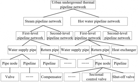
Starting from the boiler rooms, heating centers, power plants, and other heat sources, the multiple sets of pipes leading to the thermal entrance of buildings form the thermal pipeline network, whose structure is given in Figure 1.
Figure 1. Structure of urban underground thermal pipeline network
According to heat source, the urban underground thermal pipeline network can be divided into two types: the steam pipeline network, and the hot water pipeline network. Then, according to the level of the pipes, the pipeline network can be sub-divided into the first-level supply-return pipeline network from heat source to heating station, and the second-level supply-return pipeline network from heating station to heat source. For the urban thermal pipelines buried in soil, the heat transfer path during operation is: inside the pipe – inner wall of the pipe – insulation layer – outer wall of the pipe – surrounding soil. To simplify the heat calculation and the solution steps of the working process of thermal pipelines, the thermal contact resistance of the pipelines can be ignored. Suppose OI, OA, and OT are the equivalent thermal resistance values of the composite insulation layer of the pipeline, the air layer, and the soil, when calculating the temperature and heat loss of the outer protective steel pipe of the pipelines, the three kinds of thermal resistance can be added and taken as the total thermal resistance of the pipeline:
$O=O_{I}+O_{A}+O_{T}$ (1)
Suppose r represents the temperature in the pipeline, t is time, η is thermal conductivity, σ is density, ψ is specific heat capacity, and Ψ represents the heat flow for per unit volume, then a differential equation of pipeline heat conduction can be constructed as shown below:
$\frac{\partial r}{\partial t}=\frac{\eta}{\sigma \psi}\left(\frac{\partial^{2} t}{\partial a^{2}}+\frac{\partial^{2} t}{\partial b^{2}}+\frac{\partial^{2} t}{\partial c^{2}}\right)+\frac{\Psi}{\sigma \psi}$ (2)
Suppose lCI and lIS respectively represent the outer diameter of the composite insulation layer and the outer diameter of the inner steel pipe; then the equivalent thermal resistance of the composite insulation layer can be calculated by Formula 3:
$O_{I}=\frac{1}{2 \pi \eta} \ln \frac{l_{C I}}{l_{I S}}$ (3)
Suppose BP and lOS respectively represent design buried depth of the pipeline and the outer diameter of the outer protective steel pipe, ηT represents the thermal conductivity of the soil, then the equivalent thermal resistance of the soil can be calculated by Formula 4:
$O_{T}=\frac{1}{2 \pi \eta_{T}} \ln \frac{B_{P}}{l_{O S}}$ (4)
Suppose RPW and RT respectively represent the temperature of the urban underground pipeline network data matching model the temperature of the soil, then the heat loss for per unit pipe length can be calculated by Formula 5:
$J=\frac{R_{P W}-R_{T}}{O_{I}+O_{A}+O_{T}}$ (5)
Formula 6 calculates ROS, the outer surface temperature of the outer protective steel pipe of the pipeline:
$R_{O S}=R_{P W}-J\left(O_{I}+O_{A}\right)$ (6)
2.2 Calculation of stress field
The fracture of pipeline materials is mostly caused by the first two of the three common stresses of the primary stress, secondary stress, and peak stress. This paper adopted the ANSYS finite element analysis software to simulate the first two stresses, summarize the rule of stress distribution, and find out the maximum stress points of the pipeline; then the calculated values and the standard values were compared to check whether the stress tolerance range of the pipeline meets the requirements.
(1) Internal stress
Suppose LE and LN respectively represent the outer diameter and inner diameter of the pipeline, L is the diameter of the pipeline at the calculation point, F is the internal pressure of the pipeline. According to material mechanics, when thermal pipeline is subjected to internal pressure, the radial normal stress τJT of the pipeline can be calculated by Formula 7:
$\tau_{J T}=\frac{L_{N}^{2} F}{L_{E}^{2}-L_{N}^{2}}\left(1-\frac{L_{E}^{2}}{L^{2}}\right)$ (7)
The circumferential normal stress τZT of the pipeline can be calculated by Formula 8:
$\tau_{Z T}=\frac{L_{N}^{2} F}{L_{E}^{2}-L_{N}^{2}}\left(1+\frac{L_{E}^{2}}{L^{2}}\right)$ (8)
The axial normal stress τAT of the pipeline can be calculated by Formula 9:
$\tau_{A T}=\frac{L_{N}^{2} F}{L_{E}^{2}-L_{N}^{2}}$ (9)
If the thermal pipeline is regarded as thin-walled, the relevant assumptions in the thin-walled cylinder theory such as the stress along the circumferential direction is uniformly distributed along the wall, the radial stress of the pipe is zero, and the pressure load acts on the average diameter, can be applied to the scenarios of the thermal stress status analysis of pipelines. Suppose d represents the average thickness of the pipeline, then based on above assumptions, Formulas 8 and 9 can be simplified to:
$\tau_{Z T}=\frac{F L}{2 d}$ (10)
$\tau_{A T}=\frac{F L}{2 d}$ (11)
(2) Thermal stress
For multi-layer thermal pipelines of different structures, there’re differences in the temperature distribution, the temperature of the working pipelines and the external protective pipelines is uniform, and the temperature of the insulation layer of the pipelines changes linearly along the thickness direction.
Figure 2. Schematic diagram of pipelines being subject to heat and pressure
First, the condition under uniform temperature was analyzed. Suppose the two ends of the pipe are constrained by rigid walls and can stretch freely when heated, S and K respectively represent the cross-sectional area and length of the pipeline, δ and β respectively represent the elastic modulus and thermal expansion coefficient of the pipe material; if the assumptions are true, the elongation of the pipeline caused by heating expansion when the temperature rising from r1 to r2 can be calculated by Formula 12:
$\Delta K_{A}=\beta K\left(r_{2}-r_{1}\right)=\beta K \Delta r$ (12)
Figure 2 gives a schematic diagram of pipelines being subject to heat and pressure. According to the figure, as the temperature rises, the length change of the pipeline which is elongated by heating but shortened by the pressure applied by rigid walls can be calculated by Formula 13:
$\Delta K_{F}=-\frac{F_{A} K}{\delta S}$ (13)
That is, the sum of the temperature effect and the rigid wall pressure on both sides is zero, and the length of the thermal pipe remains unchanged:
$\Delta K_{A}+\Delta K_{F}=0$ (14)
Then the axial force of the pipeline can be calculated by Formula 15:
$F_{A}=\frac{\Delta K_{A}}{K} \delta S=\delta S \beta \Delta r$ (15)
Because the thermal stress of the heating expansion of the pipeline and the force FA are in an equilibrium state, namely:
$\tau_{1}=-\delta \beta \Delta r$ (16)
According to above formula, when solving the thermal stress of pipelines, since the thermal stress of the pipeline structure will increase with the rise of temperature, and at the same time this thermal stress is proportional to the elastic modulus and thermal expansion coefficient of the pipe material, it’s necessary to comprehensively consider physical relations such as the Hooke's law and the law of deformation caused by thermal expansion and contraction.
Suppose insulation cotton and air layer are the main components of the insulation layer of thermal pipelines, the thermal stress formula when the pipeline temperature changes linearly in the insulation cotton can be described by Formula 17:
$\left\{\begin{array}{c}\tau_{J T}=\frac{\beta \delta \Delta r_{i}}{2(1-\lambda) \ln \frac{L_{E}}{L_{N}}}\left[-\ln \frac{L_{E}}{L}-\frac{L_{N}^{2}}{L_{E}^{2}-L_{N}^{2}}\left(1-\frac{L_{E}^{2}}{L^{2}}\right) \ln \frac{L_{E}}{L_{N}}\right] \\ \tau_{Z T}=\frac{\beta \delta \Delta r_{i}}{2(1-\lambda) \ln \frac{L_{E}}{L_{N}}}\left[1-\ln \frac{L_{E}}{L}-\frac{L_{N}^{2}}{L_{E}^{2}-L_{N}^{2}}\left(1+\frac{L_{E}^{2}}{L^{2}}\right) \ln \frac{L_{E}}{L_{N}}\right] \\ \tau_{A T}=\frac{\alpha \delta \Delta r_{i}}{2(1-\lambda) \ln \frac{L_{E}}{L_{N}}}\left[1-2 \ln \frac{L_{E}}{L}-\frac{L_{N}^{2}}{L_{E}^{2}-L_{N}^{2}} \ln \frac{L_{E}}{L_{N}}\right]\end{array}\right.$ (17)
(3) External load stress
For thermal pipeline acting as the force-bearing structure, suppose the property of forces acting on each part of the pipeline are the same and the soil around the pipe has isotropic characteristics, then for soil under different depth D, there is:
$\tau_{D}=\sigma_{1} g D_{1}+\sigma_{2} g D_{2}+\ldots+\sigma_{M} g D_{M}=\sum_{1}^{M} \sigma_{i} g D_{i}$ (18)
Suppose ST is the linear stiffness of the soil, then the lateral stress of the soil weight can be calculated by Formula 19:
$\tau_{a}=S T_{0} \tau_{D}$ (19)
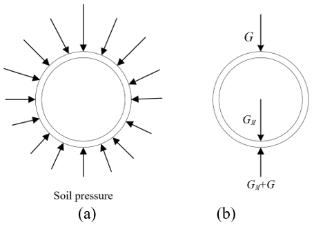
Figure 3. Stress generated by external loads acting on the pipeline
Figure 3 shows the stress of external load (soil weight) on the pipeline. Suppose G and σT represent the weight and density of soil above per unit length pipe, D represents the depth from the top of the pipe to the soil surface, then the sum of G and GM (the weight of medium contained in per unit length pipe) can be defined as the normal pressure of the soil on the pipeline, G can be calculated by Formula 20:
$G=\sigma_{T} g L_{E} D$ (20)
Suppose σP and σM represent the density of the pipe and the density of medium contained in the pipe, then GM can be calculated by Formula 21:
$G_{M}=\pi \sigma_{P} g L r+\frac{\pi}{4} L^{2} \sigma_{M} g$ (21)
The axial frictional resistance of the pipeline is:
$f_{A}=\mu\left(G+G_{M}\right)$ (22)
Soil would exert a counteracting thrust on pipeline that moves in the lateral direction to hinder its movement; based on ST, we can construct a model for the displacement of thermal pipelines and the surrounding soil, ST and the maximum thrust of the soil TH can be calculated by Formula 23:
$\left\{\begin{array}{l}S T=\frac{100}{3} \sigma_{T} g\left(D+L_{E}\right) \tan ^{2}\left(45+\frac{\Psi}{2}\right) \\ T H=\frac{100}{3} \sigma_{T} g\left(D+L_{E}\right)^{2} \tan ^{2}\left(45+\frac{\Psi}{2}\right)\end{array}\right.$ (23)
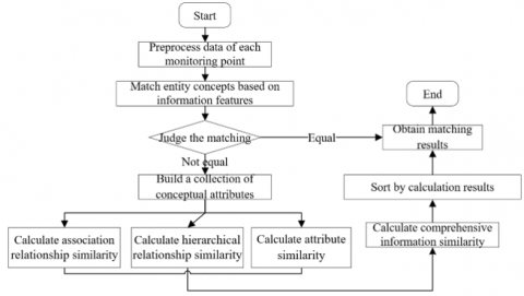
The node points in the underground thermal pipeline network actually exist and they can provide the actual hot water heating supply data, they have rich information such as associations, hierarchies, and attributes, as well as the topological information related to the distribution requirements of pipeline sections. In order to effectively make use of the node information and improve the matching efficiency and accuracy of the pipelines, this paper adopted the “node-arc” structure to describe the thermal data of the pipeline and applied the information similarity calculation method to solve the inconsistency of the information of associations, hierarchies, and attributes. The figure below gives the flow for calculating the similarity of urban underground thermal pipeline network information.
Figure 4 gives the flow of spatial data matching of urban underground thermal pipeline network. To perform spatial data matching, first, we need to measure the information similarity of each node and pipeline entity of the underground pipeline network, elements in the four contents of information expression form, information feature, correlation quantification, and correlation weight setting that are interconnected and logically progressive should be taken into consideration, on this basis, the information similarity model could be constructed to obtain the effective spatial data matching similarity.
Figure 4. Flow of spatial data matching of urban underground thermal pipeline network
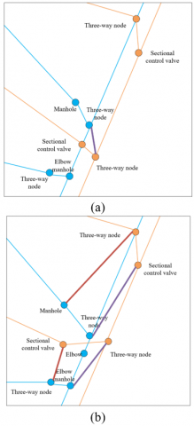
Figure 5. Differences in spatial data relationships of pipeline network
Figure 5 shows a schematic diagram of the differences in the spatial data relationship of the pipeline network. Suppose DN represents the conceptual name of the sets of nodes or pipeline entities with same information features; TA represents the spatial association relationships of underground pipelines, including the topological relationships and the directional relationships; LS and AC represent the relatively obvious hierarchical structure information and thermal stress attribute features between underground pipeline entities after classification, then, the characteristics of the underground thermal pipeline network can be described by a quadruple QU shown as Formula 24:
$Q U=<D N, T A, L S, A C>$ (24)
Suppose ARN(X,Y), ART(X,Y), ARL(X,Y), and ARC(X,Y) respectively represent the conceptual name similarity, association relationship similarity, hierarchical relationship similarity, and attribute similarity of underground pipeline network nodes or pipeline entities; θN, θL, θC, and θT represent the corresponding weights in the information similarity, then the overall information similarity IS(X,Y) of the underground pipeline network can be calculated by Formula 25:
$I S(X, Y)=\left\{\begin{array}{c}1, A R_{N}(X, Y)=1 \\ \theta_{T} \cdot A R_{T}(A, B)+\theta_{L} \cdot A R_{L}(X, Y)+ \\ \theta_{C} \cdot A R_{C}(A, B)+\theta_{N} \cdot A R_{N}(X, Y), A R_{N}(A, B) \neq 1\end{array}\right.$ (25)
Only considering the topological relationships between pipeline and node, pipeline and pipeline, and node and node, then the ART(X,Y) in above formula can be calculated by Formula 26:
$A R_{T}(X, Y)=\left\{\begin{array}{l}0, \text { Inconsistent } \\ 1, \text { Consistent } \\ \xi, \text { Have intersection }\end{array}\right.$ (26)
According to above formula, if the association relationship between two nodes or pipeline entities is inconsistent, then ART(X,Y) is equal to 0; if the association relationship is consistent, then ART(X,Y) is equal to 1; if there’s intersection between the several association relationships of two entities, then ART(X,Y) is equal to ξ, the value range is [0,1].
The hierarchical relationship of nodes or pipeline entities can be expressed by distance FN (X, Y) in the underground pipeline network structure, FN can be described by the sum of the number of sides of the shortest path between two entities. Suppose υ represents the adjustment coefficient, then the ARL(X,Y) in Formula 25 can be calculated by Formula 27:
$A R_{L}(X, Y)=\frac{1}{F N(X, Y) \times v+1}$ (27)
Figure 6. Information similarity calculation process of urban underground thermal pipeline network
Figure 6 gives the flow for calculating the information similarity of urban underground thermal pipeline network. According to the figure, the calculation of the comprehensive information similarity can be carried out after the calculation of attribute similarity is completed. Compared with the calculation of association relationship similarity and hierarchical relationship similarity, the calculation of attribute similarity is the most complicated and is realized based on the different thermal stress attributes of the nodes or pipeline entities. The manifestations of the entities’ thermal stress attributes generally include two aspects: the temperature field and the stress field; and the two aspects have different degrees of influence on the calculation of the attribute similarity of entities. Therefore, when constructing the comprehensive attribute similarity model for nodes or pipeline entities, it’s necessary to introduce influencing factors to describe the different sources of influence. Suppose hi and θi represent the component of a thermal stress attribute item of the nodes or pipeline entities and the corresponding weight, ui represents the size of the attribute value, then the collection of the conceptual attributes of each node and pipeline entity of the underground pipeline network with the same thermal stress attribute characteristics can be defined as shown in Formula 28:
$H=\left\{\left[h_{1}, u_{1}, \theta_{1}\right],\left[h_{2}, u_{2}, \theta_{2}\right], \ldots,\left[h_{M}, u_{M}, \theta_{M}\right]\right\}$ (28)
Suppose the values of the temperature and stress fields attribute item h(h∈H) of entities X and Y in the conceptual attribute collection are represented by uXh and uYh, respectively, then the ARC(X,Y) in Formula 25 can be calculated by Formula 29:
$A R_{C}(X, Y)=\sum_{h \in H}\left(\theta_{h} \times \varepsilon_{h}^{v}\left(u_{h}^{X}, u_{h}^{Y}\right)\right)$ (29)
where, εvh (uXh,uYh) is the algorithm function of temperature and stress fields attribute type, θh is the weight of each underground pipeline network attribute of concepts X and Y. Thermal stress has an extremely important influence on the shape, size, and thermodynamic properties of the underground thermal pipeline network entities. Figure 7 gives a schematic diagram of the similarity calculation of pipeline network information. For each pipeline network entity in the figure, V={DE, FE, NV} was set as the method for calculating the similarity of thermal stress attributes of DE (deformation-type attributes), FE (function-type attributes), and NV (numerical value-type attributes).
Figure 7. Pipeline network information similarity calculation
For deformation-type attributes, the similarity between each entity attribute can be calculated by comparing the differences in the deformation of two nodes or pipeline entities. Suppose ∆de(X,Y) represents the difference in deformation of two entities caused by thermal stress, then the formula for calculating the similarity of thermal stress attribute information based on deformation-type attributes DE can be expressed as:
$\varepsilon_{h}^{D E}\left(u_{h}^{X}, u_{h}^{Y}\right)=1-\frac{\Delta d e(X, Y)}{\max (d e(X), d e(Y))}$ (30)
Function-type attributes refer to the attributes with the function levels or status of the pipeline, attributes of this type are ordered nominal attributes, that is, they describe the thermal stress limit sequence or the pressure bearing degree of high-pressure, medium-pressure, and low-pressure pipelines. Suppose IV(uXh) represents the index value of this type of attributes, IR represents the index base of the attribute value domain, then by calculating the interpolation between two index values and its ratio to the index in the attribute value range, the similarity of the attributes of this type could be calculated.
$\varepsilon_{h}^{F E}\left(u_{h}^{X}, u_{h}^{Y}\right)=1-\frac{\left|F E\left(u_{h}^{X}\right), F E\left(u_{h}^{Y}\right)\right|}{I R}$ (31)
Numerical value-type attributes use numerical values to describe the differences in the thermal stress values of different thermal pipeline entities; generally, it’s considered that the difference in the thermal stress between two entities should be less than a preset threshold:
$\varepsilon_{h}^{N V}\left(u_{h}^{X}, u_{h}^{Y}\right)=\left\{\begin{array}{l}1,\left|u_{h}^{X}, u_{h}^{Y}\right| \leq \mu \\ 0,\left|u_{h}^{X}, u_{h}^{Y}\right|>\mu\end{array}\right.$ (32)
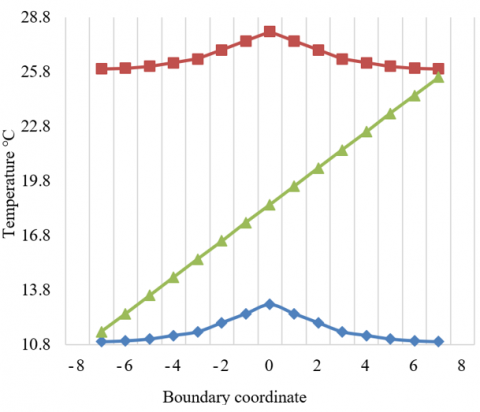
Figures 8 gives the distribution of temperature field in surrounding soil and each layer of the pipelines of the urban underground pipeline network and Figure 9 gives the corresponding simulation calculation results. According to the temperature distribution in the soil and the upper, lower, and side boundaries of the pipeline given in Figure 8, it can be seen that, when the working temperature of the pipeline was fixed at 200℃, for soil around the pipeline in the side direction, the temperature changed linearly with the change of soil depth, while in the lateral direction, the temperature in soil in upper and lower positions basically remained unchanged. Under other working temperatures, the law of temperature distribution in the soil was the same, which had verified that the soil boundary temperature is less affected by the underground pipeline network, the selection of the soil areas does not need to consider the direction factor, and the calculation results of the temperature field are reliable.
Figure 8. Temperature distribution in soil around the pipeline
Figure 9. Simulation results of pipeline temperature field under different working conditions
Figure 10. Simulation results of pipeline stress under different working conditions
Table 1. Calculation results of the similarity of the spatial structure of pipeline network nodes
|
Node pairs |
x1-x1' |
x1-x2' |
x1-x3' |
x1-x4' |
|||||
|
Similarity matrix |
Pipeline network segmentation |
x1'x2' |
x1'x3' |
x1'x4' |
x2'x1' |
x3'x1' |
x4'x1' |
x4'x5' |
x4'x5' |
|
x1x2 |
3/4 |
0 |
-3/4 |
-3/4 |
0 |
3/4 |
0 |
3/4 |
|
|
x1x3 |
0 |
1 |
0 |
0 |
-3/4 |
0 |
-2/3 |
0 |
|
|
x1x4 |
-1 |
0 |
1 |
1 |
0 |
-1 |
0 |
1 |
|
|
Information similarity |
0.872 |
0.31 |
0 |
0.35 |
|||||
According to the simulation results of the pipeline temperature field given in Figure 9, the distribution of temperature field of thermal pipelines was similar under different working temperatures, and the temperature of the inner and outer pipes were basically the same. Comparison of the simulation results of different structure schemes suggested that, changing the number and thickness of the radiation layers or changing the thickness of the air layer can both change the temperature field distribution of thermal pipelines, the insulation effect can be improved, and the temperature decreased roughly linearly with the decrease in the number and thickness of the layers. Figure 10 gives the simulation results of pipeline stress under different working conditions. Different types of L-shaped and Z-shaped pipelines, the maximum stress points were all located at the inner side of the elbow, the size of working thermal stress was less affected by medium pressure, and more affected by temperature.
Table 1 lists the calculation results of the similarity of the spatial structure of pipeline network node x1 and other nodes to be matched, it shows the proof of information similarity between the pipes associated with the pipeline network segment where the matching point x1 is located and the pipes associated with other nodes to be matched, 8 pipe pairs x1x2—x1'x2', x1x3—x1'x3', x1x4—x1'x4', x1'x4'—x2'x1', x1x4—x3'x1', x1x2—x4'x1', x1x2—x4'x5', x1x4—x4'x5' were selected for formula calculation, and the results showed that the structure similarity of pipeline network node x1 and the to-be-match node x1' was the greatest.
Figure 11 compares the matching results of urban underground pipeline network obtained by the proposed method and the traditional method. In contrast to the traditional pipeline network matching method that focuses on node information and is greatly affected by the setting of similarity weights, the method proposed in this paper started from the overall structure of the pipeline network and realized the matching of spatial data of the thermal pipeline network from both the macroscopic and the microscopic scales, and the correct rate of matching was relatively high.
Figure 11. Comparison of matching results of urban underground thermal pipeline network
Figure 12. Statistics of time cost of urban underground thermal pipeline network matching
Figure 13. Multi-process speed-up ratio of urban underground thermal pipeline network matching
Based on the MPICH2 parallel library, this study realized the development and deployment of the parallel programs for underground pipeline network matching. Figure 12 shows the time cost details of pipeline network matching in a parallel environment, and Figure 13 gives the speed-up ratio under different number of processes. The time cost of the matching of urban underground thermal pipeline network was mainly composed of two parts: the time cost of computation, and the time cost of matching, wherein the time cost of computation was inversely proportional to the number of processes, and the time cost of matching was proportional to the number of processes. The main reason is that the increase in the number of processes would increase the work load of matching. In addition, the speed-up ratio was also proportional to the number of processes.
This paper analyzed the thermal stress of urban underground pipelines and studied the matching of spatial data. The second chapter of the paper conducted theoretical analysis and simulation calculation on the temperature and stress fields of the underground pipelines and gave the simulation calculation results of internal stress, thermal stress, and external load stress. The third chapter proposed methods for information similarity calculation and spatial data matching of the underground pipelines. Then experimental results gave the temperature field distribution and simulation calculation results of pipeline layers and surrounding soil of the urban underground pipeline network, and verified the reliability of the simulation calculation results. According to the thermal stress test results of different types of L-shaped and Z-shaped pipes, this study obtained a few conclusions such as the maximum stress points were all located on the inside of the elbow, and the working thermal stress was less affected by medium pressure and more affected by temperature. At last, the matching results of urban underground pipeline network obtained by the proposed method and the traditional method were compared and the effectiveness of the spatial data matching method proposed in this paper had been proved.
This work was supported by the National Natural Science Foundation of China (No.51678226), the Natural Science Foundation of Hunan (No. 2019JJ50030), Scientific Research Project of Education Department of Hunan Province (No. 19C0358), the Science and Technology Innovation Project of Yiyang City (No. 2020YR02 and 2019YR02).
[1] Diodjo, M.T., Joliff, Y., Belec, L., Aragon, E., Perrin, F.X. (2021). Stress evolution in multilayer polymer coating under thermal and pressure loading applied to the pipeline structure. International Journal of Pressure Vessels and Piping, 191: 104386. https://doi.org/10.1016/j.ijpvp.2021.104386
[2] Drago, M., Klimenko, S., Lazzaro, C., Milotti, E., Mitselmakher, G., Necula, V., O’Brian, B., Prodi, G.A., Salemi, F., Szczepanczyk, M., Tiwari, S., Tiwari, V., Gayathri, V., Vedovato, G., Yakushin, I. (2021). Coherent WaveBurst, a pipeline for unmodeled gravitational-wave data analysis. SoftwareX, 14: 100678. https://doi.org/10.1016/j.softx.2021.100678
[3] Gong, M.X., Yuan, S., Chu, Z.W., Zhang, S.L., Fang, C.L. (2015). Underground pipeline data matching considering multiple spatial similarities. Acta Geodaetica et Cartographica Sinica, 44(12): 1392-1400. https://doi.org/10.11947/j.AGCS.2015.20150207
[4] Branowski, M., Belloum, A. (2018). Cookery: A framework for creating data processing pipeline using online services. In 2018 IEEE 14th International Conference on e-Science (e-Science), pp. 368-369. https://doi.org/10.1109/eScience.2018.00102
[5] Taler, J., Zima, W., Jaremkiewicz, M. (2016). Simple method for monitoring transient thermal stresses in pipelines. Journal of Thermal Stresses, 39(4): 386-397. https://doi.org/10.1080/01495739.2016.1152109
[6] Choi, Y.S., Chung, M.K., Kim, J.G. (2004). Effects of cyclic stress and insulation on the corrosion fatigue properties of thermally insulated pipeline. Materials Science and Engineering: A, 384(1-2): 47-56. https://doi.org/10.1016/j.msea.2004.05.068
[7] Suman, J.C., Karpathy, S.A. (1993). Design method addresses subsea pipeline thermal stresses. Oil and Gas Journal, (United States), 91(35). https://www.osti.gov/biblio/5464573
[8] Radin, Y.A., Kontorovich, T.S. (2018). An analysis of the effect of protective films on the inside surface of headers and steam pipelines in combined-cycle power plants on their thermally stressed state. Thermal Engineering, 65(10): 698-701. https://doi.org/10.1134/S0040601518100051
[9] Yan, S.W., Tian, Y.H., Liu, R., Wang, Z.L., Wang, J.Y. (2006). Analysis on interface shear stress of thermally insulated ocean pipelines under installation. China Ocean Engineering, 20(2): 315-323.
[10] Guo, L., Liu, R. (2012). High-order lateral buckling analysis of submarine pipeline under thermal stress. Transactions of Tianjin University, 18(6): 411-418. https://doi.org/10.1007/s12209-012-1867-6
[11] Mazurok, A., Vyshemirskyi, M. (201). Effect of regulation valves installation in high pressure injection system pipelines on the formation of reactor vessel thermal stress conditions. In International Conference on Nuclear Engineering, V02AT09A055. https://doi.org/10.1115/ICONE22-30437
[12] Guo, L.P., Liu, R., Yan, S.W. (2013). Global buckling behavior of submarine unburied pipelines under thermal stress. Journal of Central South University, 20(7): 2054-2065. https://doi.org/10.1007/s11771-013-1707-4
[13] Onsoien, M.I., M’hamdi, M., Akselsen, O.M. (2010). Residual stresses in weld thermal cycle simulated specimens of X70 pipeline steel. Welding Journal, 89(6): 127-132.
[14] Liu, R., Yan, S.W., Sun, G.M. (2005). Improvement of the method for marine pipeline upheaval analysis under thermal stress. Journal of Tianjin University, 38(2): 124-128.
[15] Lubecki, S., Taler, A., Sobota, T. (2008). Numerical optimization of steam pipeline heating with respect to thermal stresses. Archives of Thermodynamics, 29(4): 87-96.
[16] Belec, L., Joliff, Y. (2017). Numerical study on the evaluation of thermal and mechanical stresses during the welding of coated pipelines. Progress in Organic Coatings, 111: 336-342. https://doi.org/10.1016/j.porgcoat.2017.06.011
[17] Fang, C.L., Zhang, S.L. (2017). A concept semantic similarity method for underground pipeline spatial data matching. Journal of Computer-Aided Design and Computer Graphics, 29(4): 720-727.
[18] Hussain, M., Zhang, T., Seema, M.N., Hussain, A. (2021). Application of big data analytics to energy pipeline corrosion management. Corrosion Management, 2021: 28-29.
[19] Radin, Y.A., Kontorovich, T.S. (2021). Thermally stressed state of headers and steam pipelines in the flowpath of combined-cycle power plants during their heating with condensed steam. Thermal Engineering, 68(1): 59-64. https://doi.org/10.1134/S004060152101016X