Zhengde Wang
© 2021 IIETA. This article is published by IIETA and is licensed under the CC BY 4.0 license (http://creativecommons.org/licenses/by/4.0/).
OPEN ACCESS
In electronic equipment, thermal failure and thermal degradation are two increasingly prominent problems of the devices, with the deepening integration and growing power density. Currently, there are relatively few reports on the heat transfer mechanism, heat source analysis, and numerical simulation of electronic equipment containing power electronic devices (PEDs). Therefore, this paper carries out thermal design and evaluates the cooling performance of PED-containing electronic equipment. Firstly, the basic flow was given for the thermal design of PED-containing electronic equipment; the heat transfer mode of PEDs and the equipment were detailed, so was the principle of thermal design; the cooling principles were introduced for ventilation cooling, heat pipe cooling, and closed loop cooling. Then, numerical simulation was carried out on the solid and liquid state heat transfer of PEDs and the equipment under different cooling modes. Based on an engineering example, the cooling scheme was finalized through heat source analysis on the proposed electronic equipment. The experimental results rove the effectiveness of numerical simulation and electronic equipment cooling scheme. The results provide a reference for the cooling scheme design for other fields of thermal design.
power electronic devices (PEDs), thermal design of electronic equipment, cooling scheme
Recent years has witnessed several new trends of electronic equipment containing power electronic devices (PEDs): the widening scope of application, the diversification of functions, the rising power density, and the increasingly severe working environment. These trends pose immense challenges to the reliability design of the equipment, and the thermal design and management of the next-generation electronic systems [1-3]. Owing to the size reduction of PEDs and the growth of switching frequency, electronic equipment has become deeply integrated and dense in power. This is accompanied by the prominence of thermal failure and thermal degradation [4-6]. The thermal design of PED-containing electronic equipment requires theoretical knowledge of multiple disciplines, namely, electronics, heat transfer, mechanics, and fluid mechanics, and calls for overall consideration of the unique features in the cooling of closed equipment, which is characterized by heat concentration, a small radiating surface, and a high heat flux [7]. It is of certain practical significance to optimize the structural parameters of cooling system and the cooling conditions of electronic equipment.
Like other high-power PEDs, the insulated gate bipolar transistor (IGBT) module in dynamic reactive power compensation systems also has thermal design requirements [8, 9]. Lee et al. [10] carried out finite-element analysis on the flow field and temperature field of closed electronic equipment with radiators of different structures, and provided the steps for optimal design of water-cooling radiators.
The power increase and integration of PEDs push up the heat flux density and temperature of electronic equipment, adding to the probability of device fault and equipment failure. The situation is particularly unfavorable for closed electronic equipment working in harsh environment. Thus, it is especially important to make a reasonable and effective cooling design for electronic equipment [11-14]. Depending on the requirements of different working conditions, Alshaer et al. [15] conducted heat source analysis and thermal design for the main heating components of electronic equipment, and verified the effectiveness of the synergistic cooling scheme, which involves radiator, heat plate, and air-cooling plate, during the construction of a thermoelectric simulation network. Riehl and Cachuté [16] established a mathematical model for the heat transfer of PED fins, analyzed the cooling process and the cooling effects under different fin sizes, and realized the optimal design of fin radiator for PEDs on Simcenter Flotherm. Walsh et al. [17] studied the principle of heat pipe cooling and air-cooling plate cooling, designed a heat plate cooling scheme for electronic equipment containing digital signal processor (DSP) chip, metal-oxide-semiconductor (MOS) tube, and rectifier, calculated the parameters of the heat plate, and verified the calculation results through MATLAB simulation. Chen et al. [18] analyzed the structural displacement field, temperature field, and electromagnetic field of electronic equipment with dense heat flux, and examined the coupling relationship between multiple fields; Based on Delaunay triangulation, Chen extracted the deformation of the structural displacement field, achieved the bidirectional transmission of temperature and structure information through interpolation, and evaluated the comprehensive effects of electromagnetic compatibility and structural vibration on PED layout in the equipment.
Small electronic equipment with good cooling performance boasts a relatively wide scope of application and promising prospects of development [19]. Focusing on the high-power electronic equipment metal–oxide–semiconductor field-effect transistor (MOSFET), Fukue [20] ignored the off-state leakage current loss and drive loss, measured the steady-state power dissipation of the device, and selected the ideal radiator parameters on Simcenter Flotherm.
The current research mostly focuses on the thermal performance of the structure of multi-chip electronic equipment, the response of material parameters of devices, the estimation of equivalent thermal resistance of a single cooling scheme, and the thermal design of common forced air cooling. Few scholars have explored the heat transfer mechanism, heat source analysis, and numerical simulation of PED-containing electronic equipment. Therefore, this paper carries out thermal design of PED-containing electronic equipment, and evaluates the cooling performance of the equipment. The main aspects of this research are as follows: (1) clarifying the basic flow for the thermal design of PED-containing electronic equipment, detailing the heat transfer mode and thermal design principle of PEDs and the equipment, and introducing the principles of three common cooling modes for electronic equipment, namely, ventilation cooling, heat pipe cooling, and closed loop cooling; (2) numerically simulating the solid and liquid state heat transfer of PEDs and the equipment under different cooling modes; (3) finalizing the cooling scheme through heat source analysis on the proposed electronic equipment, in the light of an engineering example, and verifying the effectiveness of numerical simulation and electronic equipment cooling scheme through experiments.
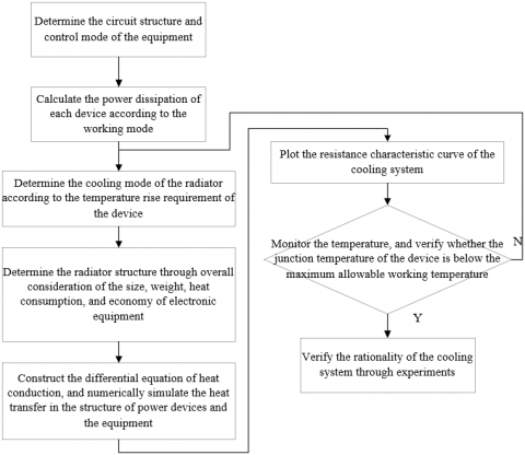
Figure 1. Basic flow of thermal design for PED-containing electronic equipment
Figure 1 shows the basic flow of the thermal design for PED-containing electronic equipment. Before the thermal design, it is necessary to get clear about the heat transfer mode of the equipment and its devices. The working process of PED-containing electronic equipment is rather complex, involving the transfer of heat, mass, and energy. Judging by the principle of heat transfer, the equipment has three basic modes of heat transfer: conduction, convection, and radiation.
The conduction of PED-containing electronic equipment can be described by Fourier’s law: during heat conduction, the temperature change rate perpendicular to the fixed cross-section and the cross-sectional area are proportional to the heat flow passing through the cross-section per unit time. Let SC be the size of the cross-section perpendicular to the heat flow direction; dΨ/da be the change rate of temperature Ψ in direction a; μ is the conduction coefficient reflecting the conduction performance of material. Then, the quantity of heat conduction QC of the electronic equipment can be calculated by:
${{Q}_{C}}=-\mu {{S}_{C}}\frac{d\psi }{da}$ (1)
where, the negative sign is the direction of temperature rise, which is opposite to the direction of heat flow. The heat convection of PED-containing electronic equipment refers to the heat transfer between the heat flow and the solid surfaces with different temperatures in contact with the flow. Let β be the heat transfer coefficient of the convection surface; SH and ΔΨ be the convection size and temperature difference between the fluid and solid surface(s), respectively. Based on Newton’s law of cooling, the quantity of heat convection QH can be calculated by:
${{Q}_{H}}=\beta {{S}_{H}}\Delta \psi $ (2)
Formula (2) shows QH and SH are positively correlated with ΔΨ; β is the proportional constant of convection.
When it comes to the heat radiation of PED-containing electronic equipment, it is known that blackbodies with an absorption ratio of 1 have a greater radiation capacity than the other objects of the same temperature. The radiating capacity of a blackbody can be calculated by adding up the radiant energies of all wavelengths in all directions of the upper part of the hemisphere centering on the blackbody from the surface area of that body in unit time. Let δb and τb be the radiation constant and absolute temperature of the blackbody, respectively. Based on Stefan-Boltzmann law, the radiating capacity Rb of the blackbody can be calculated by:
$R_{b}=\delta_{b} \psi_{b}^{4}$ (3)
Let R and σ be the thermal radiating capacity and blackness of PED-containing electronic equipment, respectively. Then, the blackness can be characterized as the ratio of R to the Rb at the same temperature:
$\sigma=R / R_{b}$ (4)
Formulas (3) and (4) can be combined into:
$R=\sigma R_{b}=\sigma \delta_{b} \psi_{b}^{4}$ (5)
PEDs generally work at high frequencies, which produces noneligible witching loss and temperature rise. Drawing on the heat transfer features of power electronic circuits, the thermal design of PED-containing electronic equipment must control the temperature of the working environment for the PEDs below the maximum allowable temperature, through the temperature control of the cooling device of the radiator. Therefore, the main purpose of the thermal design of that equipment is to create a good thermal environment on the levels of element, component, and equipment, and to ensure the reliability of electronic circuits and the effectiveness of all functions. To prepare a reasonable thermal design scheme for PED-containing electronic equipment, it is necessary to measure the parameters that induce thermal failure, and arrange devices and circuits to reduce the cooling cost, such that the electronic equipment can operate at a high reliability.
The thermal design of PED-containing electronic equipment needs to meet the maximum allowable working temperature of the equipment, the allowable power consumption of the equipment, and the limits on the cooling system, in addition to complying with other thermal environment requirements on the equipment and relevant standards. The principles for the thermal design of PED-containing electronic equipment can be summarized as follows:
(a) Give overall consideration to the size, weight, heat consumption, economy, electrical performance, and maximum allowable working temperature of each device in the equipment; the overall circuit layout; the thermal environment of equipment operation; the complexity of circuits; (b) Control temperature rise and drop of the equipment by the heat release; (c) Flexibly choose between the three heat transfer modes, namely, conduction, convection, and radiation; (d) Accurately estimate the important metrics of thermal design effectiveness, such as power consumption, thermal resistance, and temperature; (e) Select a simple, lightweight, and economic cooling device that adapts to the thermal environment of the electronic equipment; (f) After analyzing the cooling device, carry out thermal design simultaneously with the electrical design and mechanical design of the equipment; strike a balance between these designs if there is any conflict.
As can be seen from Figure 1, one of the key steps of the thermal design for PED-containing electronic equipment is to determine the cooling mode of FEDs and the equipment. The cooling mode has an immense impact on the assembly design, operational reliability, power density, and cost of the equipment. This paper introduces the principles of three common cooling modes for electronic equipment, including ventilation cooling, heat pipe cooling, and closed loop cooling.
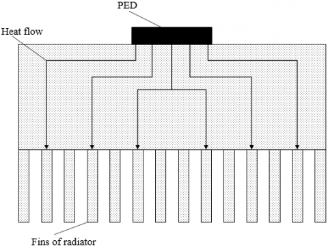
(1) Ventilation cooling
Figure 2. Principle of natural ventilation cooling of electronic equipment
Ventilation cooling can be divided into natural ventilation cooling and forced ventilation cooling. The two modes differ in temperature control requirement of the object and heat flux density. In natural ventilation cooling, the heat is transferred passively through the equipment enclosure via the three basic heat transfer modes (conduction, convection, and radiation), with the aid of the fins of the radiator. Despite the simplicity of the cooling structure, natural ventilation cooling has a low cooling efficiency, and relies too much on the cooling conditions of the equipment enclosure. Figure 2 shows the principle of natural ventilation cooling of electronic equipment. In forced ventilation cooling, the heat not dissipated by the three basic heat transfer modes is dissipated by forced ventilation, i.e., forcing the air to flow convectively. This cooling mode is very efficient in heat dissipation. However, there are several defects of forced ventilation cooling: high noise, electromagnetic interference, easy inhalation of dust, and difficulty in maintenance.
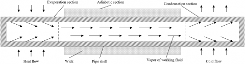
(2) Heat pipe cooling
Heat pipe cooling can be adopted, if ventilation cooling cannot fully dissipate the heat of the equipment. Figure 3 explains the principle of a common heat pipe cooling mode of electronic equipment. The heat pipe is a closed vacuum container filled with liquid medium on the inner wall. After the pipe core is heated, the liquid medium is heated to evaporation. Since the condensation section has a lower pressure than the evaporation section, the evaporated medium condensates in the condensation section under the pressure difference, and releases the latent heat of vaporization. Heat pipe cooling is known for its good cooling effect, but it is very costly and easy to pollute the environment.
Figure 3. Principle of heat pipe cooling of electronic equipment
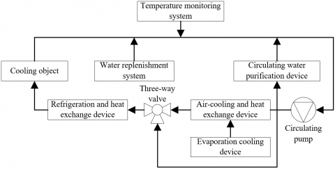
(3) Closed loop cooling
As a typical mode of closed loop cooling, circulating water cooling has always been hailed as an effective way to cool PEDs with a high power density. Figure 4 shows the principle of the closed loop cooling of electronic equipment. After being pressurized by the circulating pump, the circulating water flow takes away the remaining heat of the PEDs along the channel. The temperature of the circulating water flow is regulated by the proportional control of the water heat exchanger through the three-way valve in the water flow loop. There are several severe problems with circulating water cooling, such as the low purity of the circulating water, poor reliability, and serious corrosion. During the thermal design, the designer must treat the components of the circulating water flow and the material of the water flow loop, and automatic replenish the water loss in the loop.
Figure 4. Principle of closed loop cooling of electronic equipment
Let фM and υM be the density and specific heat of the PED material, respectively; h be the time; la, lb, and lc be the heat conduction coefficients of the material in the directions a, b, and c, respectively; ФHW be the heat flow generated the heat source within the micro-elements, i.e., the PEDs. For the three-dimensional (3D) heat transfer problem of the PED-containing electronic equipment, the transient temperature field variable Ψ(a,b,c,h) of the equipment in the rectangular coordinate system must satisfy the heat conduction differential equation:
$\begin{align} & {{\Phi }_{M}}{{\upsilon }_{M}}\frac{\partial \tau }{\partial h}-\frac{\partial }{\partial a}\left( {{l}_{a}}\frac{\partial \tau }{\partial a} \right)-\frac{\partial }{\partial b}\left( {{l}_{b}}\frac{\partial \tau }{\partial b} \right) \\ & -\frac{\partial }{\partial c}\left( {{l}_{c}}\frac{\partial \tau }{\partial c} \right)-{{\Phi }_{H}}W=0 \\\end{align}$ (6)
Formula (6) shows that the heat needed to increase the temperature of PEDs equals the superposition of the heats transmitted into the micro-elements along directions a, b, and c, with the heat generated by the heat source within the micro-elements.
Let Ma, Mb, and Mc be the directional cosines of the normal outside the boundaries, respectively; ψ1, ψ2, and ψ3 be the given temperatures on the boundaries Λ1, Λ2, and Λ3, respectively (ψ3 represents the temperature of the adiabatic wall on the boundary layer under forced ventilation, or the external environment temperature under natural ventilation); e be the heat transfer coefficient. Then, the boundary conditions that the temperature field distribution in the solution domain Γ must satisfy the given temperatures ψ1(Λ,h), ψ2(Λ, h), and ψ3(Λ, h) on boundaries Λ1, Λ2, and Λ3 can be respectively expressed as:
$\psi ={{\psi }_{1}}\left( \Lambda ,h \right) $ (7)
${{l}_{a}}\frac{\partial \psi }{\partial a}{{M}_{a}}+{{l}_{b}}\frac{\partial \psi }{\partial b}{{M}_{b}}+{{l}_{c}}\frac{\partial \psi }{\partial c}{{M}_{c}}={{\psi }_{2}} \left( \Lambda ,h \right) $ (8)
${{l}_{a}}\frac{\partial \psi }{\partial a}{{M}_{a}}+{{l}_{b}}\frac{\partial \psi }{\partial b}{{M}_{b}}+{{l}_{c}}\frac{\partial \psi }{\partial c}{{M}_{c}}=e\left( {{\psi }_{3}}-\psi \right)$ (9)
The boundaries Λ1, Λ2, and Λ3 must satisfy:
${{\Lambda }_{1}}+{{\Lambda }_{2}}+{{\Lambda }_{3}}=\Lambda $ (10)
The boundary condition (7) is a coercive condition belonging to the first kind; the boundary condition (8) is a natural adiabatic condition at ψ2=0, belonging to the second kind; boundary condition (9) is a natural condition, belonging to the third kind.
When the temperature change of a device is zero in a direction, formula (6) can be simplified to a second-order heat balance equation:
$\begin{align} & {{\Phi }_{M}}{{\upsilon }_{M}}\frac{\partial \psi }{\partial h}-\frac{\partial }{\partial a}\left( {{l}_{a}}\frac{\partial \psi }{\partial a} \right) \\ & -\frac{\partial }{\partial b}\left( {{l}_{b}}\frac{\partial \psi }{\partial b} \right)-{{\Phi }_{H}}W=0 \\\end{align}$ (11)
In this case, the two-dimensional (2D) field variable ψ(a,b,h) is no longer a function in the direction with zero temperature change. The boundary condition can be updated into:
$\psi ={{\psi }_{1}}\left( \Lambda ,h \right)$ (12)
${{l}_{a}}\frac{\partial \psi }{\partial a}{{M}_{a}}+{{l}_{b}}\frac{\partial \psi }{\partial b}{{M}_{b}}={{\psi }_{2}}\left( \Lambda ,h \right)$ (13)
${{l}_{a}}\frac{\partial \psi }{\partial a}{{M}_{a}}+{{l}_{b}}\frac{\partial \psi }{\partial b}{{M}_{b}}=e\left( {{\psi }_{3}}-\psi \right)$ (14)
Solving the transient temperature field of PED-containing electronic equipment is to solve the field function ψ that characterizes the relationship between coordinates and time under the initial conditions of h=0 and ψ=ψ0. The ψ needs to satisfy the transient heat balance equation and its corresponding boundary.
Suppose the given boundary temperatures ψ1, ψ2, and ψ3 and internal thermal energy W are constant. Then, the temperature at any point in the electronic equipment can stabilized at a fixed value after thermal exchange, that is:
$\frac{\partial \psi }{\partial h}=0$ (15)
At this time, the heat balance equation can characterize the heat conduction of the electronic equipment in steady state. In other words, the differential equation of heat conduction can be rewritten as (16) under the condition (15):
$\begin{align} & \frac{\partial }{\partial a}\left( {{l}_{a}}\frac{\partial \psi }{\partial a} \right)-\frac{\partial }{\partial b}\left( {{l}_{b}}\frac{\partial \psi }{\partial y} \right) \\ & +\frac{\partial }{\partial c}\left( {{l}_{c}}\frac{\partial \psi }{\partial c} \right)+{{\Phi }_{H}}W=0 \\\end{align}$ (16)
Under the steady state, the second-order heat balance equation can be expressed as:
$\frac{\partial }{\partial a}\left( {{l}_{a}}\frac{\partial \psi }{\partial a} \right)-\frac{\partial }{\partial b}\left( {{l}_{b}}\frac{\partial \psi }{\partial b} \right)+{{\Phi }_{H}}W=0\text{ }$ (17)
There are no relatively moving devices, when solving the problem of solid heat conduction in electronic equipment. The temperature distribution of solid media like wires, and the heat flow between media can be calculated based on the given initial and boundary conditions. Comparatively, the heat conduction problem of the fluid medium in the water cooling dissipator of power devices is relatively complicated and difficult to solve. The problem needs to be solved comprehensively by coupling the mass equation, the momentum equation, and the energy equation. Assuming that water cooling is a relatively slow forced convection under constant properties, the velocity field of the fluid medium can be calculated first.
First, it is necessary to set up a spatial rectangular coordinate system with three axes a, b, and c. Let va, vb, and vc be the velocities of the fluid medium in the three directions, respectively. Then, the water medium in the water cooling dissipator can be described by the 3DNavier-Strokes equation. In this case, the water medium is treated as an incompressible viscous fluid. Then, a continuity equation can be established under the spatial rectangular coordinate system:
$\frac{\partial {{v}_{a}}}{\partial a}+\frac{\partial {{v}_{b}}}{\partial b}+\frac{\partial {{v}_{c}}}{\partial c}=0$ (18)
Let фL be the liquid density; C be the mean hourly pressure; εa, εb, and εc be the components of gravitational acceleration in the three directions, respectively; α be the kinematic viscosity. Then, the momentums of the fluid medium in directions a, b, and c can be respectively expressed as:
$\begin{align} & \frac{\partial {{v}_{a}}}{\partial h}+\frac{\partial {{v}_{a}}}{\partial a}+\frac{\partial {{v}_{a}}}{\partial b}+{{v}_{c}}\frac{\partial {{v}_{a}}}{\partial c}=-\frac{1}{{{\Phi }_{L}}}\frac{\partial C}{\partial a} \\ & +{{\varepsilon }_{a}}+\alpha \left( \frac{{{\partial }^{2}}{{v}_{a}}}{\partial {{a}^{2}}}+\frac{{{\partial }^{2}}{{v}_{a}}}{\partial {{b}^{2}}}+\frac{{{\partial }^{2}}{{v}_{a}}}{\partial {{c}^{2}}} \right) \\\end{align}$ (19)
$\begin{align} & \frac{\partial {{v}_{b}}}{\partial h}+\frac{\partial {{v}_{b}}}{\partial a}+\frac{\partial {{v}_{b}}}{\partial c}+{{v}_{c}}\frac{\partial {{v}_{a}}}{\partial c}=-\frac{1}{{{\Phi }_{L}}}\frac{\partial C}{\partial b} \\ & +{{\varepsilon }_{b}}+\alpha \left( \frac{{{\partial }^{2}}{{v}_{b}}}{\partial {{a}^{2}}}+\frac{{{\partial }^{2}}{{v}_{b}}}{\partial {{b}^{2}}}+\frac{{{\partial }^{2}}{{v}_{b}}}{\partial {{c}^{2}}} \right) \\\end{align}$ (20)
$\begin{align} & \frac{\partial {{v}_{c}}}{\partial h}+\frac{\partial {{v}_{c}}}{\partial a}+\frac{\partial {{v}_{c}}}{\partial b}+w\frac{\partial {{v}_{c}}}{\partial c}=-\frac{1}{{{\Phi }_{L}}}\frac{\partial C}{\partial c} \\ & +{{\varepsilon }_{c}}+\alpha \left( \frac{{{\partial }^{2}}{{v}_{c}}}{\partial {{a}^{2}}}+\frac{{{\partial }^{2}}{{v}_{c}}}{\partial {{b}^{2}}}+\frac{{{\partial }^{2}}{{v}_{c}}}{\partial {{c}^{2}}} \right) \\\end{align}$ (21)
Let ψL, υL, and μL be the temperature, specific heat capacity, and conduction coefficient of the liquid, respectively; WE be the heat source term. Then, the energy of the fluid medium can be described as:
$\begin{align} & \frac{\partial {{\psi }_{L}}}{\partial h}+\frac{\partial {{\psi }_{L}}}{\partial a}+\frac{\partial {{\psi }_{L}}}{\partial b}+{{v}_{c}}\frac{\partial {{\psi }_{L}}}{\partial c} \\ & =\frac{1}{{{\Phi }_{L}}{{\upsilon }_{L}}}\frac{\partial }{\partial a}\left[ \mu \frac{\partial {{\psi }_{L}}}{\partial a} \right]+\frac{1}{{{\Phi }_{L}}{{\upsilon }_{L}}}\frac{\partial }{\partial b}\left[ \mu \frac{\partial {{\psi }_{L}}}{\partial b} \right] \\ & +\frac{1}{{{\Phi }_{L}}{{\upsilon }_{L}}}\frac{\partial }{\partial c}\left[ \mu \frac{\partial {{\psi }_{L}}}{\partial c} \right]+{{W}_{E}} \\\end{align}$ (22)
Based on an engineering example, the proposed electronic equipment contains the following heating components: a 12W CPU chip, an 8W DSP chip, two MOSFETs, three CPU mainboards of the rectifier module, a 45W power module, and two 13W data modules. The power losses of MOSFETs and rectifier module were estimated after consulting the data on these devices and referring to empirical values and actual working conditions (Table 1).
(1) Power loss of MOSFET
MOSFET is a classic switching PED. The power loss of MOSFET consists of on-state loss LOSSC and switching loss LOSSS. Let ID, rD, and Dmax be the on-state current, on-state resistance, and maximum duty cycle of MOSFET, respectively. Then, LOSSC can be calculated by:
$LOS{{S}_{C}}=I_{D}^{2}\times {{r}_{D}}\times {{D}_{max}}$ (23)
Let UI be the input voltage, hUP be the current rise time, td (off) hDOWN be the current drop time, and fKG be the switching frequency of MOSFET, respectively. Then, LOSSS can be calculated by:
$LOS{{S}_{S}}=\frac{1}{2}{{U}_{I}}{{I}_{D}}\left[ {{h}_{UP}}+{{h}_{DOWN}} \right]{{f}_{KG}}$ (24)
(2) Power loss of rectifier
In the proposed electronic equipment, each set of rectifier contains 4 diodes. Without considering wire loss, all the loss of the rectifier comes from the 4 diodes. Let DD, UZ, and IZ be the duty cycle, forward voltage drop, and forward on-state current of the diodes, respectively. Then, the forward on-state power loss LOSSD of the diodes can be calculated by:
$LOS{{S}_{D}}=D\times {{I}_{Z}}\times {{U}_{Z}}$ (25)
Based on the working principle of the electronic equipment, and the calculated power losses of the main heating components, the cooling problems of the electronic equipment, which consists of a power module, data modules, a CPU chip, a DSP chip, MOSFETs, and a rectifier module, were summarized as follows: high-power devices concentrate on the printed circuit board (PCB); with the highest power loss, the CPU gives off the greatest amount of heat; the local heat flow is very likely to become too dense. Besides, the small spacing between CPU mainboards and PCB hinder the internal air flow, causing an excessive temperature rise in the electronic equipment.
Figure 5 shows the thermoelectric simulation network of the PED-containing electronic equipment, where PC is a power component; r1, r2, r3, and r4 are the equivalent thermal resistances between PC and PCB, PCB and locking device, locking device and equipment enclosure, and equipment enclosure and surrounding environment, respectively; r5 is the radiation resistance; Ψ1 and Ψ2 are the ambient temperature and the temperature surrounding PEDs and other power devices. As shown in Figure 5, the heat of PEDs and other power devices can be transferred along three paths. Most electronic components are in a closed state, with weak convection in the internal air. Therefore, only a small quantity of heat is transferred from the electronic equipment via convection and radiation. Therefore, the thermal design of the equipment should give priority to water cooling or heat transfer via the equipment enclosure.
Table 1. Physical parameters of heating components in the electronic equipment
|
Serial number |
Name |
Power loss |
Number |
Location |
|
1 |
Data module 1 |
13 |
1 |
Middle part of equipment |
|
2 |
Data module 2 |
16 |
1 |
Middle part of equipment |
|
3 |
Power module |
50 |
1 |
Bottom of equipment |
|
4 |
Rectifier |
1.85 |
3 |
Mainboard |
|
5 |
MOSFET |
2.09 |
2 |
Mainboard |
|
6 |
DSP |
7 |
1 |
Mainboard |
|
7 |
Central processing unit (CPU) |
11 |
1 |
Mainboard |
Figure 5. Thermoelectric simulation network of the PED-containing electronic equipment
Using the key points of Simcenter Flotherm, the PED-containing electronic equipment was meshed into grids for thermal simulation. Figure 6 presents the temperature curves of the main heating components in the proposed electronic equipment. It can be seen that the heating power devices are densely distributed around the CPU, emitting lots of heat in local areas. The temperatures of CPU module, DSP chip, and power module all rose by more than 130°C. For the diode-containing rectifier and MOSFETs, the temperature rises were 100°C above the upper limit of working temperature. Therefore, necessary measures should be taken to ensure the cooling requirements of the proposed closed electronic equipment for normal operation.
Figure 6. Temperature curves of main heating components of the electronic equipment
According to the principle of natural ventilation cooling for PED-containing electronic equipment, the cooling effect of the fins in the radiator is greatly affected by the surface heat transfer coefficient, fin height, and fin thickness. This paper optimizes the natural ventilation cooling scheme by adjusting fin height, fin number, and fin thickness. Taking PED temperature as the objective function, 15 natural ventilation cooling schemes were solved based on Command Center module. The results in Table 2 show that the cooling module of natural ventilation cooling should not be too large, due to the limitations of internal space, power density, and cooling efficiency of the proposed electronic equipment; if it is difficult to meet the requirements on thermal design, the cooling module can be directly connected with the equipment enclosure via heat pipes to reduce thermal resistances like r1, r2, r3, and r4, thereby cooling down the chips.
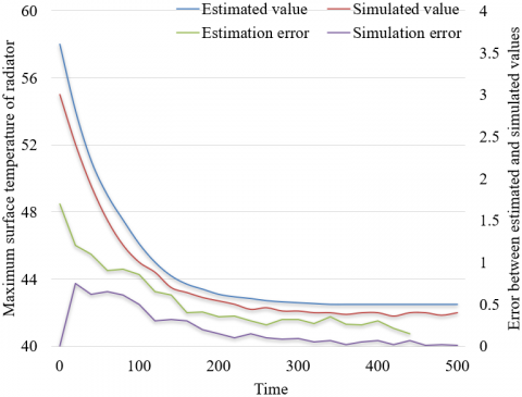
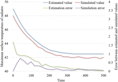
To further examine the influence of each thermal design scheme on the temperature rise and cooling effect of PEDs, this paper estimates the maximum surface temperature of the cooling module based on the calculated power losses of MOSFETs and rectifier (Section 4), and compares the estimated result with the result of transient thermal simulation on Ansys Icepak. Figures 7 and 8 display the temperature rise and error curves under the MOSFET power loss of 250W and 100W, respectively. Under the two power losses, the estimated maximum surface temperature of the cooling module was basically the same as the simulated results, with a calculation error within 4%. The maximum temperature difference between estimated and simulated results was about 3.8℃.
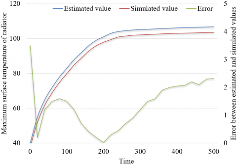
Figures 9 and 10 display the temperature drop and error curves under the MOSFET power loss of 250W and 100W, respectively. Comparing the temperature rise and temperature drop curves under the same power loss, it can be inferred that the surface temperature of the cooling module peaked at 53.2℃ and 47.9℃, respectively, during the temperature rise after the steady-state heat balance; the lower bounds of the maximum surface temperature of the cooling module stood at 44.9℃ and 45.3℃, respectively, during the temperature drop. As shown in Figures 9 and 10, under the two power losses, the estimated maximum surface temperature of the cooling module was basically the same as the simulated results, with a calculation error within 5%. The maximum temperature difference between estimated and simulated results was about 2.5℃.
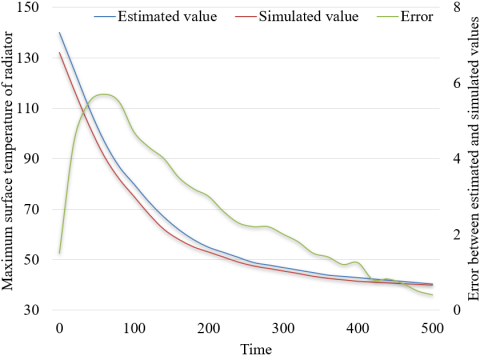
When the electronic equipment has overcurrent, the heat loss of each device will increase instantly. Figures 11 and 12 show the curves of temperature rise and temperature drop, as well as corresponding errors of the cooling module under overcurrent, respectively. The estimated maximum surface temperature of the cooling module was compared with the result of transient thermal simulation on Ansys Icepak. The calculation error (<5%) and maximum temperature difference (4.7℃) were both within the allowed ranges. This further indicates that our calculation method for power loss applies to the overcurrent condition of the electronic equipment; our calculation and simulation strategies can respond to the maximum surface temperature of the cooling module dynamically and accurately.
Table 2. Simulation results of natural ventilation cooling schemes
|
Scheme number |
Fin height |
Fin number |
Fin thickness |
Component temperature |
|
1 |
10.9 |
7 |
0.72 |
115.2 |
|
2 |
13 |
6 |
0.69 |
119.5 |
|
3 |
17.1 |
9 |
0.67 |
107.3 |
|
4 |
18.9 |
7 |
0.55 |
109.9 |
|
5 |
22.3 |
8 |
1.03 |
101.6 |
|
6 |
23 |
6 |
1.01 |
109.4 |
|
7 |
22.5 |
9 |
1.42 |
103 |
|
8 |
23.7 |
6 |
0.55 |
115.8 |
|
9 |
25.6 |
7 |
0.97 |
101 |
|
10 |
27 |
9 |
0.63 |
105.3 |
|
11 |
25.9 |
7 |
0.55 |
109.5 |
|
12 |
28.1 |
6 |
1.36 |
101.7 |
|
13 |
28.9 |
11 |
1.2 |
103 |
|
14 |
30.1 |
9 |
1.35 |
97.53 |
|
15 |
29.8 |
4 |
0.83 |
109.1 |
Besides, it can be observed that the surface temperature of the cooling module reached 70.2℃, after the electronic equipment remained in overcurrent state for 1min. However, that temperature should not surpass 70℃ for the safe and reliable operations of MOSFET with the power loss of 250W. Thus, the proposed electronic equipment can only work for 45-50s under overcurrent. The longest working time of MOSFET should be estimated by the above analysis approach, trying to prevent MOSFET from being burnt through long-term operation under overcurrent.
This paper mainly carries out thermal design and evaluate the cooling performance of PED-containing electronic equipment. After introducing the basic flow of thermal design, the authors provided the details on the heat transfer modes of PEDs and the equipment, and clarified the cooling principles of three common cooling modes. Then, numerical simulation was carried out on the solid and liquid heat transfer process of PEDs and electronic equipment under each cooling mode. Combining an engineering example, the heat source analysis was performed on the proposed electronic equipment to determine the final cooling scheme. By adjusting three variables (fin height, fin number, and fin thickness), the natural ventilation cooling scheme was optimized, and the influence of the scheme on temperature rise and drop of PEDs was investigated step by step. The experimental results show that our calculation and simulation strategies can respond to the maximum surface temperature of the cooling module dynamically and accurately; our numerical simulation and cooling scheme were effective for the proposed electronic equipment.
[1] Pan, H., Ma, L., Zhu, L., Wang, H. (2020). Thermal design of electronic equipment based on parametric simulation. Proceedings of the Seventh Asia International Symposium on Mechatronics, Singapore, pp. 319-325. https://doi.org/10.1007/978-981-32-9441-7_32
[2] Tariq, S.L., Ali, H.M., Akram, M.A., Janjua, M.M. (2020). Experimental investigation on graphene based nanoparticles enhanced phase change materials (GbNePCMs) for thermal management of electronic equipment. Journal of Energy Storage, 30: 101497. https://doi.org/10.1016/j.est.2020.101497
[3] Cheli, L., Carcasci, C. (2020). Modelling and analysis of a liquid-cooled system for thermal management application of an electronic equipment. E3S Web of Conferences, 197: 10008. https://doi.org/10.1051/e3sconf/202019710008
[4] Kitamura, Y., Ishizuka, M., Nakagawa, S. (2006). Study on the chimney effect in natural air-cooled electronic equipment casings under inclination: Proposal of a thermal design correlation that includes the porosity coefficient of an outlet opening. Heat Transfer-Asian Research: Co-sponsored by the Society of Chemical Engineers of Japan and the Heat Transfer Division of ASME, 35(2): 122-136. https://doi.org/10.1002/htj.20103
[5] Shilo, G., Ogrenich, E., Kulyaba-Kharitonova, T., Buhaiev, O. (2019). Thermal design of the electronic equipment enclosures with natural air cooling. 2019 9th International Conference on Advanced Computer Information Technologies (ACIT), pp. 153-156. https://doi.org/10.1109/ACITT.2019.8780110
[6] Chen, B. (2013). Thermal design, analysis and experimental verification of electronic equipment of a satellite borne microwave radiometer. Advanced Materials Research, 655: 84-87. https://doi.org/10.4028/www.scientific.net/AMR.655-657.84
[7] Ishizuka, M., Hatakeyama, T., Kibushi, R. (2013). A thermal design approach for natural air cooled electronic equipment casings. 2013 8th International Microsystems, Packaging, Assembly and Circuits Technology Conference (IMPACT), pp. 67-70. https://doi.org/10.1109/IMPACT.2013.6706631
[8] Koizumi, K. (2015). Thermal simulation techniques for the design of power electronics equipment. Journal of Japan Institute of Electronics Packaging, 18(2): 100-103. https://doi.org/10.5104/jiep.18.100
[9] Fukue, T., Ishizuka, M., Nakagawa, S., Hatakeyama, T., Koizumi, K. (2011). Model for predicting performance of cooling fans for thermal design of electronic equipment (Modeling and evaluation of effects from electronic enclosure and inlet sizes). Heat Transfer-Asian Research, 40(4): 369-386. https://doi.org/10.1002/htj.20347
[10] Lee, D.K., Lee, W.H., Park, S.W., Kang, S.W., Cho, J.H. (2017). Numerical analysis for thermal design of electronic equipment using phase change material. Transactions of the Korean Society of Mechanical Engineers B, 41(4): 285-291. https://doi.org/10.3795/KSME-B.2017.41.4.285
[11] Wang, L., Li, L.M., Zeng, G.Q., Sun, J.L., Wu, L., Wang, H., Dai, Y.X. (2017). Thermal sturcutre design of air-cooled heat sinks for power electronic equipments by constrained population extremal optimization. 2017 Chinese Automation Congress (CAC), pp. 2467-2472. https://doi.org/10.1109/CAC.2017.8243190
[12] Yokono, Y., Hisano, K., Hirohata, K. (2009). Categorized application technology of numerical simulation on electronic equipment thermal design. International Electronic Packaging Technical Conference and Exhibition, 43604: 247-252. https://doi.org/10.1115/InterPACK2009-89057
[13] Nakamura, H. (2009). Cooling fan model for thermal design of compact electronic equipment: Improvement of modeling using PQ Curve. International Electronic Packaging Technical Conference and Exhibition, 43604: 221-228. https://doi.org/10.1115/InterPACK2009-89010
[14] Kafadarova, N., Stoyanova, D., Stoyanova-Petrova, S., Mileva, N., Vakrilov, N. (2019). Our experience in using performance support learning in “thermal management of electronic equipment” course. 2019 IEEE XXVIII International Scientific Conference Electronics (ET), pp. 1-4. https://doi.org/10.1109/ET.2019.8878599
[15] Alshaer, W.G., Nada, S.A., Rady, M.A., Le Bot, C., Del Barrio, E.P. (2015). Numerical investigations of using carbon foam/PCM/Nano carbon tubes composites in thermal management of electronic equipment. Energy Conversion and Management, 89: 873-884. https://doi.org/10.1016/j.enconman.2014.10.045
[16] Riehl, R.R., Cachuté, L.D.O. (2014). Thermal management of surveillance equipments electronic components using pulsating heat pipes. Fourteenth Intersociety Conference on Thermal and Thermomechanical Phenomena in Electronic Systems (ITherm), pp. 513-518. https://doi.org/10.1109/ITHERM.2014.6892324
[17] Walsh, E., Walsh, P., Grimes, R., Egan, V. (2008). Thermal management of low profile electronic equipment using radial fans and heat sinks. Journal of Heat Transfer, 130(12): 125001. https://doi.org/10.1115/1.2977602
[18] Chen, L.H., Wu, Q.W., Luo, Z.T., Dong, J.H., Jiang, F. (2009). Design for thermal control system of electronic equipment in space camera. Optics and Precision Engineering, 17(9): 2145-2152.
[19] Fukue, T., Ishizuka, M., Hatakeyama, T., Nakagawa, S., Koizumi, K. (2011). Study on PQ curves of cooling fans for thermal design of electronic equipment (Effects of opening position of obstructions near a fan). Fluids Engineering Division Summer Meeting, 44403:. 737-745. https://doi.org/10.1115/AJK2011-22054
[20] Fukue, T. (2018). Novel development for thermal design of electronic equipment using pulsating flow from knowledge of nature. Journal of Japan Institute of Electronics Packaging, 21(2): 114-121. https://doi.org/10.5104/jiep.21.114