Yanán Camaraza-Medina
© 2021 IIETA. This article is published by IIETA and is licensed under the CC BY 4.0 license (http://creativecommons.org/licenses/by/4.0/).
OPEN ACCESS
This paper presents the main results of the research developed by the author in his postdoctoral investigations on heat transfer calculations during film condensation inside tubes. The elements studied are combined in an analysis expression that provides a reasonable fit with the available experimental data, which includes a total of 22 fluids, including water, refrigerants and a wide range of organic substances, which condense inside horizontal, inclined and vertical tubes. These experimental data were obtained from the reports of 33 sources. Available data covers tube diameters from 2 to 50 mm, mass flow rates from 3 to 850 kg/(m2s), reduced pressures $p_{r}=P / P_{c}$ ranging from 0.0008 to 0.91, Pr values for single-phase from 1 to $20 \times 10^{3}$, Reynolds number for two-phase from 900 to 594390, Reynolds number for single-phase from 65 to 84950 and vapor quality from 0.01 to 0.99. The mean deviation found for the analyzed data for horizontal tubes was 13.4%, while for the inclined and vertical tubes data the mean deviation was 14.9%. In all cases, the agreement of the proposed model is good enough to be considered satisfactory for practical design.
film condensation, heat transfer coefficient, adimensional velocity, mathematical deduction
In the modern engineering, it is possible to find in advanced literature, an important group of papers in which the heat transfer inside tubes is reviewed or studied. However, the characteristics of the heat transfer process in tubes and the elements related to it generate a complex analysis process, being required in all cases of experimentation and model correlation. In the last five decades an important group of methods and models have been presented, which have been validated from available experimental data.
Several specialized studies, Camaraza-Medina et al. [1], Boyko and Kruzhilin [2], Rabiee et al. [3], Zeinelabdeen et al. [4], Lee et al. [5] have provided a detailed analysis of several models of wide diffusion and acceptance, being widely discussed, their ability to predict the average heat transfer coefficients. However, the literature lacks a single criterion that establishes the suitable dimensionless groups to build a model for the determination of heat transfer coefficients in film condensation.
Most of the known models use approximately five to ten dimensionless groups and validation and adjustment parameters, however, they have a common point, and it consists in the use of the Dittus-Boelter model for the calculation of the heat transfer coefficients in single-phase, which only includes two dimensionless groups and three adjustment values. This model is given by Chen et al. [6], Shah [7, 8]:
$N u_{L}=\frac{h d}{k}=c R e^{m} P r^{n}$ (1)
where, h is the single-phase heat transfer coefficient, d is the inner diameter of tube, k is the fluid thermal conductivity, $\operatorname{Re}=G d / \mu$ is the Reynolds number, (with G being the mass flux and $\mu$ the dynamic viscosity), $P r=\mu c_{p} / k$ is the Prandtl number. The exponent n is suggested to be 0.3 and 0.4 for cooling and heating respectively, while $m=0.8 \text { and } c=0.023 .$
The present research includes high and low mass flows, with the objective that the developed model can consider and predict the effects associated with stratification. An important group of experimental data reported by various authors was collected, in which various tube diameters and various fluid properties are included.
This paper presents the main results of the research developed by the author in his postdoctoral investigations. The elements studied are combined in an analysis expression that provides a reasonable fit with the available experimental data, which includes a total of 22 fluids, including water, refrigerants and a wide range of organic substances. These experimental data were obtained from the reports of 33 sources. Available data covers tube diameters from 2 to 50 mm, mass flow rates from 3 to 850 kg/(m2s), and reduced pressures $p_{r}=P / P_{c}$ ranging from 0.0008 to 0.91.
The main objective of this paper is to define and identify the dimensionless groups that allow the heat transfer coefficient to be described more adequately during film condensation inside tubes, in addition to developing a mathematical procedure that generates a new, improved model for calculating the heat transfer coefficients during film condensation inside tubes.
If in a tube a three-dimensional control volume is taken inside and it is also considered that the heat flux by conduction cannot be neglected, then, the equation for the conservation of energy applied to the analyzed tube is described by [9]:
$\rho C_{p} \frac{\partial T}{\partial t}=\frac{\partial}{\partial x}\left(k \frac{\partial T}{\partial x}\right)+\frac{\partial}{\partial y}\left(k \frac{\partial T}{\partial y}\right)+\frac{\partial}{\partial z}\left(k \frac{\partial T}{\partial z}\right)$ (2)
The energy equation for the fluid is described by:
$\begin{aligned}
\rho c\left[\frac{\partial T}{\partial \tau}+V_{x} \frac{\partial T}{\partial x}+V_{y}\right.&\left.\frac{\partial T}{\partial y}+V_{z} \frac{\partial T}{\partial z}\right] \\
&=k\left(\frac{\partial^{2} T}{\partial x^{2}}+\frac{\partial^{2} T}{\partial y^{2}}+\frac{\partial^{2} T}{\partial z^{2}}\right)+\mu \Phi
\end{aligned}$ (3)
In Eq. (3), the viscous cutting effects are considered by means of the Schlichting function of viscous dissipation $\Phi$ [4]:
$\Phi=2\left[\left(\frac{\partial V_{x}}{\partial x}\right)^{2}+\left(\frac{\partial V_{y}}{\partial y}\right)^{2}+\left(\frac{\partial V_{z}}{\partial z}\right)^{2}\right]+\left(\frac{\partial V_{x}}{\partial x}+\frac{\partial V_{y}}{\partial y}+\frac{\partial V_{z}}{\partial z}\right)^{2}$ (4)
The viscous dissipation function is considered because it can generate a very important influence on high velocity flows. The compressibility of the flow is present due to the existence of a phase change, for this reason it is necessary to consider the density variations associated with the phase change. The process can be considered as continuous, therefore the continuity equation is:
$\frac{\partial \rho}{\partial \tau}+\frac{\partial\left(\rho V_{x}\right)}{\partial x}+\frac{\partial\left(\rho V_{y}\right)}{\partial y}+\frac{\partial\left(\rho V_{z}\right)}{\partial z}=0$ (5)
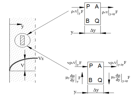
In the tube, an elemental section is taken as a control volume (see Figure 1). In this analysis, the flow is assumed to be one-dimensional, so the directional transport effects along the tube (axial) are more important than the radial ones. Therefore, Eqns. (2), (3), (4) and (5) can be simplified to expressions (6), (7), (8) and (9):
One-dimensional energy equation. for the tube
$\rho c_{p} \frac{\partial T}{\partial \tau}=\frac{\partial}{\partial x}\left(k \frac{\partial T}{\partial x}\right)$ (6)
One-dimensional energy equation. for the fluid
$\rho c\left[\frac{\partial T}{\partial \tau}+V_{x} \frac{\partial T}{\partial x}\right]=k\left(\frac{\partial^{2} T}{\partial x^{2}}\right)+\mu \Phi$ (7)
One-dimensional function of the viscous dissipation term
$\Phi=3\left(\frac{\partial V_{x}}{\partial x}\right)^{2}$ (8)
One-dimensional continuity equation
$\frac{\partial \rho}{\partial \tau}+\frac{\partial\left(\rho V_{x}\right)}{\partial x}=0$ (9)
In Figure 1, assuming that the heat exchange process is stationary, segments PB and AQ are the respective inputs and outputs of the heat flow to the analyzed control volume in the PB and AQ segments the heat transfer process can be described by means of an unknown functional, described by the following relationships:
$\left\{\begin{array}{ll}
x=X_{1}(t) & \text { for } P B \\
x=X_{2}(t) & \text { for } A Q
\end{array}\right.$ (10)
The mathematical axiom of the maximum value generates that the analyzed problem has a univocal and continuous solution throughout its interval. For this purpose, the Eq. (6) is applied, obtaining that the Green differential is:
$\Xi_{(T)}=-a^{2} \frac{\partial^{2} T}{\partial x^{2}}+\frac{\partial T}{\partial t}$ (11)
Figure 1. Elementary volume used in the analyzed problem
The elemental control volume PAQB is divided into four sub-elements PB, AQ, BQ and AP. Therefore, for each segment, the integration of the differential Eq. (6) and its homogeneous combination to Green's Integral produces as a result a complex integral that includes the sum of four integral relations, one for each sub-element respectively [10, 11]:
$\begin{array}{c}
\int_{P B} \varphi \psi d x-\int_{A Q} \varphi \psi d x+\int_{B Q}[\varphi \psi d x \\
\left.+a^{2}\left(\psi \frac{\partial \varphi}{\partial x}-\varphi \frac{\partial \psi}{\partial x}\right) d t\right] \\
-\int_{A P}\left[\varphi \psi d x+a^{2}\left(\psi \frac{\partial \varphi}{\partial x}-\varphi \frac{\partial \psi}{\partial x}\right) d t\right]=0
\end{array}$ (12)
In Eq. (12) the term $\varphi(x, t)$ is the solution for heat transfer process.
If the Green functional is equated to zero, then the source function $\psi=G_{0}(x, t, \xi, \tau)$ is generated. This equation can be expressed in terms of infinite line as:
$\psi=G_{0}(x, t, \xi, t)=\frac{1}{2 \sqrt{\pi a^{2}(t-\tau)^{2}}} e^{-\frac{(x-\xi)^{2}}{4 a^{2}(t-\tau)}}$ (13)
The solution for heat transfer process $\varphi(x, t)$ is obtained in the elementary volume PAQB, assuming that in the inward contour of the control volume the solution of the heat transfer problem is given by $\varphi(x, t+h), \text { where } h>0$. Substituting $x-h=\xi \text { and } t=\tau+h$, then Eq. (13) is transformed to:
$\psi=G_{0}(x, t)=\frac{1}{2 \sqrt{x a^{2} h^{2}}} e^{-\frac{(2 x-h)}{4 a^{2} h}}$ (14)
$\int_{P B} \varphi(x, t) \frac{1}{2 \sqrt{\pi a^{2} h^{2}}} e^{\frac{(2 x-h)^{2}}{4 a^{2} h}} d x-\int_{A Q} \varphi(x, t) \frac{1}{2 \sqrt{\pi a^{2} h^{2}}} e^{-\frac{(2 x-h)^{2}}{4 a^{2} h}} d x-$
$+\int_{B Q}\left[\varphi(x, t) \frac{1}{2 \sqrt{\pi a^{2} h^{2}}} e^{-\frac{(2 x-h)^{2}}{4 a^{2} h}} d x+a^{2}\left(\frac{1}{2 \sqrt{\pi a^{2} h^{2}}} e^{-\frac{(2 x-h)^{2}}{4 a^{2} h}} \frac{\partial \varphi(x, t)}{\partial x}-\varphi(x, t) \frac{\partial\left(\frac{1}{2 \sqrt{\pi a^{2} h^{2}}} e^{-\frac{(2 x-h)^{2}}{4 a^{2} h}}\right)}{\partial x}\right) d t\right]-$ (15)
$+\int_{A P}\left[\varphi(x, t) \frac{1}{2 \sqrt{\pi a^{2} h^{2}}} e^{-\frac{(2 x-h)^{2}}{4 a^{2} h}} d x+a^{2}\left(\frac{1}{2 \sqrt{\pi a^{2} h^{2}}} e^{-\frac{(2 x-h)^{2}}{4 a^{2} h}} \frac{\partial \varphi(x, t)}{\partial x}-\varphi(x, t) \frac{\partial\left(\frac{1}{2 \sqrt{\pi a^{2} h^{2}}} e^{-\frac{(2 x-h)^{2}}{4 a^{2} h}}\right)}{\partial x}\right) d t\right]=0$
Applying the limit when $h \rightarrow 0$ in Eq. (14), considering that is a continuous function. The obtained result is substituted into Eq. (12), then, Eq. (15) is generated.
Eq. (15) is very complex, and its solution by traditional integration methods would require considerable time and greater rigor. However, this difficulty can be overcome if numerical solution techniques are used, among them the benefits provided by the finite element method (FEM). For this purpose, we start from the criterion that by means of FEM techniques, it is possible to obtain a weak solution of the problem studied. For this purpose, the minimum energy principle is applied on the control volume PABQ, which is equivalent to finding a minimum of the integral complex shown in Eq. (15). For this purpose the following substitutions are required:
$\bar{\omega} \varphi(x, t) \frac{1}{2 \sqrt{\pi a^{2} h^{2}}} e^{-\frac{(2 x-h)^{2}}{4 a^{2} h}}=\bar{\omega}$ (16)
or:
$\begin{array}{l}
\frac{1}{2 \sqrt{\pi a^{2} h^{2}}} e^{-\frac{(2 x-h)^{2}}{4 a^{2} h}} \frac{\partial \varphi(x, t)}{\partial x} \\
-\varphi(x, t) \frac{\partial\left(\frac{1}{2 \sqrt{\pi a^{2} h^{2}}} e^{\left.-\frac{(2 x-h)^{2}\quad}{4 a^{2} h}\right)}\right.}{\partial x}=\omega
\end{array}$ (17)
That proves to be equivalent:
$\bar{\omega} \frac{\partial \varphi}{\partial x}-\varphi(x, t) \frac{\partial \bar{\omega}}{\partial x}=\omega$ (18)
Substituting Eq. (18) and Eq. (16), into Eq. (15):
$\begin{array}{c}
\int_{P B} \bar{\omega} d x-\int_{A Q} \bar{\omega} d x+\int_{B Q}\left[\bar{\omega} d x+a^{2}\left(\bar{\omega} \frac{\partial \varphi(x, t)}{\partial x}\right.\right. \\
\left.\left.-\varphi(x, t) \frac{\partial \bar{\omega}}{\partial x}\right) d t\right] \\
-\int_{A P}\left[\bar{\omega} d x+a^{2}\left(\bar{\omega} \frac{\partial \varphi(x, t)}{\partial x}-\right.\right. \\
\left.\left.-\varphi(x, t) \frac{\partial \bar{\omega}}{\partial x}\right) d t\right]=0
\end{array}$ (19)
With the application of FEM techniques, Eq. (19) can be transformed into a local domain, which in turn would be integrated of two linear elements composed of three nodes each (one-dimensional quadratic element). If second order parabolic arcs are used instead of linear segments in the free meshing adjustment, it is possible to obtain a more cautious approximation for the temperature distribution profile. The one-dimensional element used (see Figure 2), has a node at each end and a third node located in the center of the element [9, 10].
Figure 2. One-dimensional element (quadratic)
For these elements, the form functions are given by:
$N_{1}=-\frac{1}{2} \xi(1-\xi) ; N_{2}=(1+\xi)(1+\xi)$; $N_{3}=\frac{1}{2} \xi(1+\xi)$ (20)
The nodal solutions $N_{1}, N_{2} \text { and } N_{3}$ combined in the form of a product generate a weak function, which allows describing the temperature field and its distribution $d x d \tau$ by conduction along the axial dimension $d x$. Applying the substitution $x-h=\xi$ and assuming the extreme limit when $h=0$, then, this transformation allows us to reach the term a $x=\xi$. Therefore, three quadratic elements are possible, which is equivalent to having three work zones [11]:
$N_{1}=-\frac{1}{2} x+x^{2} ; N_{2}=1+2 x+x^{2}$; $N_{3}=\frac{1}{2} x+x^{2}$ (21)
If the variable dependence with time is unknown, then it is required to use the simplified energy equation, Eq. (3), and substitute it in the parabolic function present in the nodal solution. This technique is necessary for each integral element of the simplified Eq. (19), then:
Segment PB
Entry
$\left(-\frac{1}{2} x+x^{2}\right) V_{X}=a\left(-\frac{1}{2} x+x^{2}\right)^{2}+3 \mu\left(\frac{\partial V_{X}}{\partial x}\right)^{2}$ (22)
Intermediate
$\left(1-2 x+x^{2}\right) V_{x}=a\left(1-2 x+x^{2}\right)^{2}+3 \mu\left(\frac{\partial V_{X}}{\partial x}\right)^{2}$ (23)
Exit
$\left(\frac{1}{2} x+x^{2}\right) V_{X}=a\left(\frac{1}{2} x+x^{2}\right)^{2}+3 \mu\left(\frac{\partial V_{X}}{\partial x}\right)^{2}$ (24)
Segment AQ
Entry
$-\left(-\frac{1}{2} x+x^{2}\right) V_{X}=-a\left(-\frac{1}{2} x+x^{2}\right)^{2}+-3 \mu\left(\frac{\partial V_{X}}{\partial x}\right)^{2}$ (25)
Intermediate
$-\left(1+2 x+x^{2}\right) V_{x}=-a\left(1+2 x+x^{2}\right)^{2}-3 \mu\left(\frac{\partial V_{X}}{\partial x}\right)^{2}$ (26)
Exit
$-\left(\frac{1}{2} x+x^{2}\right) V_{X}=-a\left(\frac{1}{2} x+x^{2}\right)^{2}-3 \mu\left(\frac{\partial V_{X}}{\partial x}\right)^{2}$ (27)
When reviewing the control volume, it is verified that the sides BQ and AP do not include vertical components, however, if they consider the infinite source function, Eq. (14), for which it is required that the variation of physical properties a along the nodal segment are subordinate to the continuity equation, Eq. (9). The density changes as the length of the tube increases, due to the phase change and the compressibility of the vapor. If the process is considered as stationary, then $\partial \rho / \partial \tau=0$, therefore, Eq. (9) is transformed to [12]:
$\frac{\partial\left(\rho V_{x}\right)}{\partial x}=0$ (28)
If vapor density at the inlet is called $\rho_{V}$, and liquid density at the outlet is called $\rho_{L}$. Then, when checking the viscous stress diagram (see Figure 1), two fundamental forces are distinguished, the first associated with the drag of the vapor and the second is linked to the gravitational force, while in the opposite direction the effect of viscous forces (friction) appears. As the entire heat transfer process happens in a continuous, confined and oriented medium, then the velocity variation depends on a characteristic dimension of the duct, so it can be established that the differential Eq. (27) can be transformed to generate the relationship that allows evaluating the velocity profile (differential equation of the velocity profile), and that is also valid for any section of the conduit examined, this is:
$\mu_{L} \frac{\partial^{2} V}{\partial x^{2}}+\left(\rho_{L}+\rho_{V}\right) g=0$ (29)
In Eq. (29), $V(x)$ is the velocity through the film, for any value of x. To solve this problem, two boundary conditions are required. On the wall the condition of non-slip fluid is applied, therefore:
$x=0 \text { and } V=0$ (30)
On the film surface, the vapor drag is assumed can be despised. If the function $\delta(x)$ is considered to be the thickness of the film, the required boundary condition will then be as follows:
$x=\delta ; \frac{\partial V}{\partial x}=0$ (31)
The condensate film thickness $\delta(x)$ has not been determined. Considering that the vapor drag is negligible can be a valid assumption on many occasions; however, it is applicable only when the vapor velocity is not very high. By integrating the differential Eq. (29), the following is obtained [13, 14]:
$\frac{\partial V}{\partial x}=-\frac{\left(\rho_{L}-\rho_{V}\right) g \sin \theta}{\mu_{L}}+C_{1}$ (32)
Applying in Eq. (32) the condition of contour given in Eq. (31), then:
$0=-\delta \frac{\left(\rho_{L}-\rho_{V}\right) g \sin \theta}{\mu_{L}}+C_{1}$ (33)
Solving the integration constant $C_{1}$ in Eq. (33):
$C_{1}=\delta \frac{\left(\rho_{L}-\rho_{V}\right) g \sin \theta}{\mu_{L}}$ (34)
Replacing Eq. (34) and the contour condition given in Eq. (31) into Eq. (32)
$\frac{\partial V}{\partial x}=\frac{\left(\rho_{L}-\rho_{V}\right) g \sin \theta}{\mu_{L}}(\delta-x)$ (35)
Integrating again the differential Eq. (33) gives:
$V=\frac{\left(\rho_{L}-\rho_{V}\right) g \sin \theta}{\mu_{L}}\left(\delta x-\frac{x^{2}}{2}\right)+C_{2}$ (36)
Using the boundary condition stated in Eq. (31) and substituting it into Eq. (36) leads to $C_{2}=0$. Reordering Eq. (36) later:
$V=\delta^{2} \frac{\left(\rho_{L}-\rho_{V}\right) g \sin \theta}{\mu_{L}}\left[\frac{x}{\delta}-\frac{1}{2}\left(\frac{x}{\delta}\right)^{2}\right]$ (37)
Eq. (37) shows that the velocity profile $V(x)$ is parabolic. The velocity will have a maximum value on the surface of the film when $x=\delta$. Therefore, the maximum velocity can be obtained, if the boundary condition given in Eq. (31) is substituted in Eq. (37), then [15]:
$V_{M a x}=\delta^{2} \frac{\left(\rho_{L}-\rho_{V}\right) g \sin \theta}{2 \mu_{L}}=\frac{g \delta^{2} \sin \theta}{2 v_{L}} \frac{\left(\rho_{L}-\rho_{V}\right)}{\rho_{L}}$ (38)
Replacing Eq. (35) in Eq. (28):
$\frac{\left(\rho_{L}-\rho_{V}\right) g \sin \theta}{\mu_{L}}(\delta-x)=0$ (39)
Therefore, the arbitrary function $\varphi(x, t)$ that was assumed to establish the solution of the thermal exchange problem, takes into account the variation of the velocity profile along the characteristic length of the conduit examined.
If additionally, it is considered that the arbitrary function $\varphi(x, t)$ is similar in its numerical and functional value to Eq. (39), then, in the third and fourth terms of Eq. (19) the arbitrary function $\varphi(x, t)$ can be replaced by Eq. (37). Integrating:
$\begin{array}{l}
\bar{\omega} x+\left\{\frac{\partial}{\partial x}\left[\frac{a^{2} t \bar{\omega}\left(\rho_{L}-\rho_{V}\right) g \sin \theta\left(\delta^{2}-x\right)}{\mu_{L}}\right]+\right. \\
\left.-\frac{a^{2} t\left(\rho_{L}-\rho_{V}\right) g \sin \theta}{\mu_{L}}\left(\delta^{2}-x\right) \frac{\partial \bar{\omega}}{\partial x}\right\}-\frac{1}{2} \bar{\omega} x+ \\
+a^{2} t\left[\frac{\bar{\omega} \frac{\left(\rho_{L}-\rho_{V}\right) g \sin \theta}{\mu_{L}}\left(\delta^{2}-x\right)}{\partial x}-\right. \\
\left.-\frac{\left(\rho_{L}-\rho_{V}\right) g \sin \theta}{\mu_{L}}\left(\delta^{2}-x\right) \frac{\partial \bar{\omega}}{\partial x}\right]
\end{array}$ (40)
When the velocity is a maximum, then the equality $x=\delta$ is fulfilled. Applying this equality in Eq. (38):
$\begin{aligned}
\bar{\omega} & x^{2}+\frac{a^{2} t \bar{\omega}\left(\rho_{L}-\rho_{V}\right) g \sin \theta}{\mu_{L}}-\\
&-\bar{\omega} \frac{a^{2} t\left(\rho_{L}-\rho_{V}\right) g \sin \theta}{\mu_{L}}+\\
+& \frac{a^{2} t \bar{\omega}\left(\rho_{L}-\rho_{V}\right) g \sin \theta}{\mu_{L}}-\bar{\omega} x+\\
+& \frac{a^{2} t \bar{\omega}\left(\rho_{L}-\rho_{V}\right) g \sin \theta}{\mu_{L}}=0
\end{aligned}$ (41)
Simplifying Eq. (41)
$\bar{\omega} x^{2}-\bar{\omega} x=0$ (42)
Eq. (42) turns out to be identical to the term that describes the input discretization in the nodal distribution, therefore, the remaining nodal combinations (two) are applicable to the two finite elements that cover the horizontal segments, and the node effect initial in the third and fourth terms of Eq. (19) can be neglected. For this reason, it can be established that these initial nodes are stationary or origin points, therefore:
Segment BQ
Entry
$V_{X}=a x+3 \mu x\left(\frac{\partial V_{X}}{\partial x}\right)^{2}$ (43)
Intermediate
$\begin{array}{l}
\left(1+2 x+x^{2}\right) V_{x}=a x\left(1+2 x+x^{2}\right)^{2}+ \\
+3 \mu x\left(\frac{\partial V_{X}}{\partial x}\right)^{2}
\end{array}$ (44)
Exit
$\left(\frac{1}{2} x+x^{2}\right) V_{X}=a x\left(\frac{1}{2} x+x^{2}\right)^{2}+3 \mu x\left(\frac{\partial V_{X}}{\partial x}\right)^{2}$ (45)
Segment AP
Entry
$-V_{X}=-a x-3 \mu\left(\frac{\partial V_{X}}{\partial x}\right)^{2}$ (46)
Intermediate
$\begin{array}{c}
-\left(1+2 x+x^{2}\right) V_{X}=-a x\left(1+2 x+x^{2}\right)^{2}+ \\
-3 \mu x\left(\frac{\partial V_{X}}{\partial x}\right)^{2}
\end{array}$ (47)
Exit
$-\left(\frac{1}{2} x+x^{2}\right) V_{x}=-a x\left(\frac{1}{2} x+x^{2}\right)^{2}-3 \mu x\left(\frac{\partial V_{X}}{\partial x}\right)^{2}$ (48)
Substituting Eq. (43) into Eqns. (35) and (37) gives:
$\begin{aligned}
\delta^{2} \frac{\left(\rho_{L}-\rho_{V}\right) g \sin \theta}{\mu_{L}}\left[\frac{x}{\delta}-\frac{1}{2}\left(\frac{x}{\delta}\right)^{2}\right]=a x+\\
+3 \mu x\left[\frac{\left(\rho_{L}-\rho_{V}\right) g \sin \theta}{\mu_{L}}(\delta-x)\right]^{2}
\end{aligned}$ (49)
$\begin{array}{l}
\frac{x \delta\left(\rho_{L}-\rho_{V}\right) g \sin \theta}{\mu_{L}}-\frac{x^{2}\left(\rho_{L}-\rho_{V}\right) g \sin \theta}{2 \mu_{L}} \\
=a x+3 \mu x\left[\frac{\left(\rho_{L}-\rho_{V}\right) g \sin \theta}{\mu_{L}}(\delta-x)\right]^{2}
\end{array}$ (50)
Grouping and reducing similar terms in Eq. (50):
$(\delta-x)=a+\left(3 \mu x^{2}+\frac{\delta^{2}}{x}-2 \delta\right)\left[\frac{\left(\rho_{L}-\rho_{V}\right) g \sin \theta}{\mu_{L}}\right]$ (51)
As x is the characteristic dimension, then, $x=r=d / 2$. Substituting this term into Eq. (51):
$\begin{aligned}
\left(\delta-\frac{d}{2}\right)=& a+\left[3 \mu\left(\frac{d}{2}\right)^{2}+\frac{2 \delta^{2}}{d}-2 \delta\right] . \\
&\left[\frac{\left(\rho_{L}-\rho_{V}\right) g \sin \theta}{\mu_{L}}\right]
\end{aligned}$ (52)
Solving for the diameter in Eq. (52)
$d=2 \delta-2 a-\left(1.5 \mu d^{2}+\frac{4 \delta^{2}}{d}-4 \delta\right)\left[\frac{\left(\rho_{L}-\rho_{V}\right) g \sin \theta}{\mu_{L}}\right]$ (53)
Eq. (53) is a transcendent type Equation, and allows obtaining the required duct diameter for a pre-established flow of condensate through a horizontal tube, in order to avoid fluid stagnation. In a horizontal tube $\theta=0^{\circ} ; \text { therefore, } \sin \theta=0$ and the Eq. (53) can be simplified, obtaining:
$d=2 \delta-2 a$ (54)
or:
$x=2(\delta-a)$ (55)
If V_X≈V Max is considered, Eq. (38) now becomes [16]:
$V_{X}=\frac{g d^{2} \sin \theta}{2 v_{L}} \frac{\left(\rho_{L}-\rho_{V}\right)}{\rho_{L}}$ (56)
The velocity gradient is described by Eq. (35), in which the velocity profile was assumed for the analysis as parabolic. If additionally, it is considered that the maximum velocity is obtained in the intermediate node, then Eqns. (55), (56) and (57) are substituted in the intermediate segment BQ (Eq. (44), obtaining Eq. (57):
Segment BQ (Intermediate)
$\begin{array}{l}
\left(1+4 \delta-4 a+4 \delta^{2}-8 a \delta+4 a^{2}\right) \frac{g \delta^{2} \sin \theta}{2 v_{L}} \frac{\left(\rho_{L}-\rho_{V}\right)}{\rho_{L}} \\
=\left(2 a \delta-2 a^{2}\right) \cdot\left(1+4 \delta-4 a+4 \delta^{2}-8 a \delta+4 a^{2}\right)^{2} \\
+(6 \mu \delta-6 \mu a)\left[\frac{\left(\rho_{L}-\rho_{V}\right) g \sin \theta}{\mu_{L}}(2 a-\delta)\right]^{2}
\end{array}$ (57)
Reducing similar terms in Eq. (57):
$\begin{array}{c}
\frac{\left(\rho_{L}-\rho_{V}\right) g \delta^{2} \sin \theta}{2 \mu_{L}} \\
\frac{(6 \mu \delta-6 \mu a)\left[\frac{\left(\rho_{L}-\rho_{V}\right) g \sin \theta}{\mu_{L}}(2 a-\delta)\right]^{2}}{\left(1+4 \delta-4 a+4 \delta^{2}-8 a \delta+4 a^{2}\right)}+ \\
-\frac{\left(1+4 \delta-4 a+4 \delta^{2}-8 a \delta+4 a^{2}\right)}{=\left(2 a \delta-2 a^{2}\right)}
\end{array}$ (58)
Eq. (58) is a weak solution for the nodal discretization developed to establish the nodal distribution of the condensate at the midpoint of the horizontal control volume. When the velocity is lower, it is satisfied that $\delta \approx 0$, therefore, Eq. (58) becomes:
$\frac{(6 \mu a)\left[\frac{2 a\left(\rho_{L}-\rho_{V}\right) g \sin \theta}{\mu_{L}}\quad\right]^{2}}{\left(1-4 a+4 a^{2}\right)}=2 a^{2}$ (59)
From Eq. (55):
$a=\frac{x}{2}-\delta=\frac{d}{4} ; \quad \Rightarrow \quad x=\frac{d}{2} ; \delta=0$ (60)
Substituting Eq. (60) into Eq. (59) and simplifying:
$\frac{\left[d\left(\rho_{L}-\rho_{V}\right) g \sin \theta\right]^{2}}{\sqrt{6 \mu}\left(\mu_{L} d^{2}-\mu_{L} d\right)^{2}}=0$ (61)
The basic problem is studied for vertical installations, therefore, for horizontal tubes $\theta=90^{\circ}$, then $\sin \theta=1$. Transforming conveniently in Eq. (61) and applying radicals’ properties, then:
$\frac{\sqrt{g d\left(\rho_{L}-\rho_{V}\right)}}{6 \mu}=0$ (62)
where, 6μ is the viscous dissipation function [17]. The viscous dissipation term is the quotient between the density of the vapor and the mass flow:
$6 \mu=G / \rho_{V}^{0.5}$ (63)
The effect generated by variation of the thermodynamic vapor quality $x^{\prime}$, is included in the viscous dissipation criteria [9-11], then Eq. (61) is transformed to:
$6 \mu=G x / \rho_{V}^{0.5}$ (64)
Replacing Eq. (64) into Eq. (62):
$\frac{\sqrt{g d \rho_{V}\left(\rho_{L}-\rho_{V}\right)}}{x G}=0$ (65)
The dimensionless parameter shown in Eq. (65) was generated with the use of weak formulations, applying FEM techniques. The dimensional parameter given by Eq. (65) is known as dimensionless velocity (1/J_g) and is an essential and required element for the description and prediction of film condensation inside tubes [18-20].
$J_{g}=\frac{x G}{\sqrt{g d \rho_{V}\left(\rho_{L}-\rho_{V}\right)}}$ (66)
For vertical and inclined tubes, the application of weak solutions leads to a result identical to that obtained in Eq. (66) [21-23]. A criterion currently accepted is the use of the Shah parameter to define the prevailing condensation regime [8], establishing that three types of thermal regimes are possible inside vertical and inclined tubes. The parameter given by Shah is described by means of the following expression:
$Z=\left(\frac{1-x}{x}\right)^{0.8} \operatorname{Pr}_{L}^{0.4}$ (67)
Condensation inside tubes is governed and directly conditioned by two dimensionless parameters, Eqns. (66) and (67) [24-26]. The finite element evaluated, for the case of vertical and inclined geometric configuration, is made up of three nodes; therefore, it is required to identify the three regions generated for this purpose. However, for horizontal configurations, the intermediate node is suppressed, causing only two regions to be required. To define the validity range of each zone for the case of inclined and vertical tubes, (see Figure 1) it is assumed that the flow enters the elementary section through segment PB and leaves this section through segment QA.
To define the validity range of zone 1, two input nodes in segments PB and AQ must be taken into account. For the first, Eqns. (35), (38) and (55) are substituted in Eq. (22), while for the second we proceed in the same way with Eqns. (35), (38) and (55), those that are substituted in Eq. (25). The two new expressions obtained are added and subsequently the value of this sum is equated with Eq. (64), solving this equality as a function of dimensionless velocity.
To define the validity range of zone 2, two intermediate nodes in the PB and AQ segments must be taken into account. For the first, Eqns. (35), (38) and (55) are substituted in Eq. (23), while for the second one proceeds in the same way with Eqns. (35), (38) and (55), those that are substituted in Eq. (26). The two new expressions obtained are added and subsequently the value of this sum is equated with Eq. (64), solving this equality as a function of dimensionless velocity.
To define the validity range of zone 3, two output nodes must be taken into account in the PB and AQ segments. For the first, Eqns. (35), (38) and (55) are substituted in Equation (24), while for the second one proceeds in the same way with Eqns. (35), (38) and (55), those that are substituted in Eq. (27). The two new expressions obtained are added and subsequently the value of this sum is equated with Eq. (64), solving this equality as a function of dimensionless velocity.
The mathematical transformations required in the three previous paragraphs turn out to be extremely voluminous and complex, therefore, in the paper only the final results of the mathematical operations performed will be given [27-29]:
For vertical and inclined tubes
Zone 1 $J_{g} \geq \frac{1}{2.37 Z+0.728}$ (68)
Zone 2 $0.927 e^{\left(-0.0868 Z^{-1.165}\right)}<J_{g}<\frac{1}{2.37 Z+0.728}$ (69)
Zone 3 $J_{g} \leq 0.927 e^{\left(-0.0868 Z^{-1.165}\right)}$ (70)
To define the validity range of each zone, in the case of horizontal tubes (see Figure 1), it is assumed that the flow enters the control volume through the BQ segment and leaves it through the AP segment.
To establish the validity range of Zone 1, two input nodes are defined in the BQ and AP segments. For the first, Eqns. (35), (38) and (55) are replaced in Eq. (43), while for the second, Eqns. (36), (39) and (56) are replaced in Eq. (46). The two new relations obtained are added later and the result of the sum is equated with Eq. (64), solving this equality as a function of dimensionless velocity.
To establish the validity range of zone 2, two input nodes are defined in the BQ and AP segments. For the first, Eqns. (35), (38) and (55) are replaced in Eq. (45), while for the second; Eqns. (36), (39) and (56) are replaced in Eq. (48). The two new relations obtained are added later and the result of the sum is equated with Eq. (64), solving this equality as a function of dimensionless velocity.
The mathematical transformations required in the two previous paragraphs turn out to be extremely voluminous and complex, therefore, in the paper only the final results of the mathematical operations performed will be given [30-32]:
For horizontal pipes
Zone 1 $J_{g} \leq 0.979(Z+0.262)^{-0.618}$ (71)
Zone 2 $J_{g}>0.979(Z+0.262)^{-0.618}$ (72)
3.1 Proposal model for heat transfer evaluation during film condensation inside tubes
Validation and adjustment of the available experimental data allowed a new correlation, given by Camaraza [18]:
$N u_{T}=N u_{L}\left\{4.9 x^{0.9}\left[(1-x)^{2}+\frac{(1-x)^{0.1}}{P r^{0.37}}\right]\right\}^{0.8}$ (73)
where, NuL is given by the following Eq. [19]:
$N u_{L}=\frac{\left(R e_{L}-10^{D}\right) P r_{L}^{1.1}}{85.44 B^{2}-104 B\left(1-P r_{L}^{2 / 3}\right)}$ (74)
where,
$B=\log \left(\frac{R e_{L}^{0.56}}{3.196}\right)$;
$D=-0.0272 Y^{2}+0.2006 Y+2.6322 ;$ (75)
$Y=\log \left(R e_{L}\right)$
while, for vertical tubes $N u_{\text {vert }}$ is obtained as Medina et al. [20], Borishanskiy et al. [21]:
$N u_{\text {vert }}=0.943\left[d^{3} \frac{g\left(\rho_{L}-\rho_{V}\right) h_{f g}^{\prime}}{v_{L} k_{L}\left(T_{\text {sat }}-T_{P}\right)}\right]^{\frac{1}{4}}$ (76)
Eqns. (73) and (76) must be combined according to the zone, by means of the following procedure
For zone 1 $N u=N u_{T}$ (77)
For zone 2 $N u=\sqrt{\left(N u_{T}\right)^{2}+\left(N u_{V e r t}\right)^{2}}$ (78)
For zone 3 $N u=N u_{V e r t}$ (79)
Table 1. Validity range of the new model
|
Parameter |
Range |
|
Fluids |
Benzene, Ethanol, Ethylene glycol, Isobutene, Methanol, Propane, Propylene, Toluene R-113, R-123, R-125, R-134a, R-142b, R-22, R32, R-404a, R-410a, R-502, R-507 and Water. |
|
$J_{g}$ |
0.6 to 20 |
|
Tube inner diameter (mm) |
2 to 50 |
|
Z |
0.005 to 20 |
|
Tube orientation |
horizontal, vertical and inclined with downwards flow |
|
$\operatorname{Pr}_{L}$ |
1 to $20 \times 10^{3}$ |
|
x (steam quality) |
0.01 to 0.99 |
|
Reduced pressure, $p_{R} |
0.0008 to 0.91 |
|
$\operatorname{Re}_{V}$ |
900 to 594390 |
|
$\operatorname{Re}_{L}$ |
65 to 84950 |
|
G (kg/m2s) |
4 to 850 |
In horizontal tubes Eq. (78) is valid only for $R e \geq 3.5 \cdot 10^{4}$; for $\operatorname{Re}<3.5 \cdot 10^{4} \text { delete the term } N u_{\text {Vert }} \text { . }$ Table 1 summarizes the range for which the model developed in this investigation provides an adequate fit.
3.2 Comparison of the proposed model with experimental data and its applications
Tables 2 and 3 summarize the correlation adjustment made between the developed model and the available experimental data [2-6, 8, 10-13, 16, 17, 22-25, 33-39], which include data reported by 33 sources, covering 22 fluids, including refrigerants, various organic substances, and water. The flow rates considered range from 4 to 850 kg/m2s, with pipe diameters of 2 to 50 mm, and reduced pressure $p_{R}=P / P_{c}$ from 0.0008 to 0.91.
In the development and adjustment of this research, it was found that the experimental data showed a better behavior in the validation of the model when phase viscosity and reduced pressure were interrelated. For this reason, a correction factor is developed that includes this adjustment, which is incorporated into Eq. (73), where its constants were selected based on a statistical adjustment of trial and error in the correlation indices, using the method of Brezhnetzov.
Table 2. Comparison of Eq. (73) and experimental data for vertical and inclined tubes
|
Data Source |
Data Number |
Fluid |
Diameter (mm) |
G (kg/m2s) |
x |
$R e_{L}$ |
$\boldsymbol{R e}_{V}$ |
$\boldsymbol{p}_{r}$ |
Deviation Percent |
|
Carpenter and Colburn [9] |
18 |
Water |
11.6 |
16 180 |
0.72 0.45 |
640 26510 |
15200 130000 |
0.0046 |
21.4 -12.8 |
|
16 |
Ethanol |
11.6 |
16 140 |
0.71 0.42 |
680 6240 |
15485 134474 |
0.017 |
21.3 -14.8 |
|
|
19 |
Toluene |
11.6 |
32 154 |
0.67 0.5 |
1500 7250 |
41450 97820 |
0.025 |
22.1 -19.2 |
|
|
17 |
Methanol |
11.6 |
23 170 |
0.8 0.4 |
820 6420 |
24220 154590 |
0.016 |
20.8 -21.7 |
|
|
Gooykoontz and Dorsch [10] |
24 |
Water |
15.9 |
22 74 |
0.99 0.01 |
570 2630 |
1250 4560 |
0.005 0.017 |
17.1 -13.2 |
|
Gooykoontz and Dorsch [11] |
29 |
Water |
7.4 |
121 264 |
0.92 0.06 |
3720 6940 |
78600 167420 |
0.002 0.0062 |
13.9 -11.5 |
|
35 |
R-113 |
7.4 |
37 85 |
0.95 0.16 |
2910 5620 |
11000 19000 |
0.02 0.09 |
16.6 -19.4 |
|
|
Rosson [13] |
27 |
R-113 |
12.8 |
18 70 |
0.99 0.42 |
1100 16960 |
50800 141400 |
0.03 0.034 |
13.5 -18.6 |
|
Cavallini et al. [16] |
22 |
Benzene |
18.9 |
22 146 |
0.99 0.01 |
600 4100 |
1500 6200 |
0.02 0.021 |
11.8 -13.1 |
|
Borishanky et al. [21] |
58 |
Water |
10.0 19.3 |
10 670 |
0.8 0.39 |
760 58950 |
8100 333250 |
0.036 0.308 |
12.7 -11.3 |
|
Lee et al. [22] |
17 |
Water |
12.0 |
27 45 |
0.75 0.06 |
980 19440 |
27120 55150 |
0.0046 |
16.9 -18.1 |
|
Blageti and Slunder [23] |
24 |
Water |
30.0 |
4 69 |
0.78 0.04 |
400 7980 |
9100 252428 |
0.0046 |
22.9 -10.3 |
|
29 |
Dowtherm |
30.0 |
4 81 |
0.98 0.05 |
65 1940 |
9500 205980 |
0.008 |
19.7 -15.6 |
|
|
Ananiev et al. [24] |
111 |
Water |
8.0 50 |
30 680 |
0.99 0.01 |
1025 33120 |
21070 89880 |
0.0031 0.59 |
25.3 -20.5 |
|
Tepe and Mueller [25] |
47 |
Methanol |
18.5 |
16 30 |
0.78 0.43 |
970 5810 |
27100 50940 |
0.016 |
16.6 -10.9 |
|
119
13 |
Benzene |
18.5 |
25 66 52 88 |
0.65 0.5 0.6 0.51 |
1510 6500 3050 35000 |
49510 131420 103850 175690 |
0.021 |
14.3 -8.3 10.1 -19.2 |
|
|
Yan and Lin [26] |
26 |
R-134a |
2 |
100 200 |
0.94 0.1 |
1010 2090 |
15800 33950 |
0.16 0.32 |
13.2 -12.9 |
|
Akers et al. [27] |
35 |
Propane |
15.7 |
13 162 |
0.84 0.51 |
3800 48100 |
16530 216990 |
0.657 |
21.3 -20.6 |
|
Lemmon et al. [28] |
31 |
Water |
40.0 |
24 48 |
0.98 0.64 |
3420 6860 |
79110 159500 |
0.0046 |
12.7 -11.3 |
|
Tang [29] |
19 |
Water |
28.2 |
3 |
0.9 0.4 |
170 3540 |
8210 13480 |
0.0008 |
14.1 -12.2 |
|
Mollamahmutoglu [30] |
35 |
Water |
47.5 |
10 |
0.94 0.12 |
2550 4860 |
12880 35410 |
0.023 |
16.2 -13.6 |
|
For all sources above |
760 |
|
2 47.5 |
3 680 |
0.01 0.99 |
65 58950 |
1250 333250 |
0.0008 0.657 |
17.1 -14.7 |
Table 3. Comparison between Eq. (75) and experimental data for horizontal tubes
|
Data Source |
Data Number |
Fluid |
Diameter (mm) |
G (kg/m2s) |
x |
$\boldsymbol{R e}_{L}$ |
$\boldsymbol{R e}_{V}$ |
$\boldsymbol{p}_{r}$ |
Deviation Percent |
|
Boyko and Kruzhilin [2] |
68 |
Water |
8.0 |
38 160 |
0.99 0.01 |
1025 4324 |
21100 89100 |
0.031 0.44 |
24.1 -19.5 |
|
Carpenter and Colburn [9] |
22 |
Benzene |
18.9 |
22 146 |
0.99 0.01 |
600 2100 |
1500 5000 |
0.02 0.021 |
11.8 -10.8 |
|
Gooykoontz and Dorsch [11] |
32 |
Water |
15.9 |
20 74 |
0.99 0.01 |
660 2800 |
1320 4960 |
0.005 0.017 |
17.0 -12.4 |
|
Tandon et al. [14] |
27 |
Water |
49.0 |
12 130 |
0.95 0.54 |
1808 3450 |
54400 87950 |
0.0023 |
6.2 -9.5 |
|
Tang [29] |
56 |
R134a |
8.8 |
260 850 |
0.81 0.08 |
11560 36500 |
181800 594390 |
0.22 0.25 |
8.1 -9.3 |
|
32 |
R-410a |
8.8 |
320 720 |
0.84 0.07 |
29810 84920 |
191910 473970 |
0.46 0.5 |
16.7 -14.4 |
|
|
32 |
R-22 |
8.8 |
270 790 |
0.92 0.09 |
11520 33910 |
165740 485970 |
0.31 |
12.3 -10.9 |
|
|
Mollamahmutoglu [30] |
27 |
R-22 |
12.5 |
210 634 |
0.90 0.09 |
12550 38490 |
193600 569490 |
0.24 0.33 |
15.6 -13.7 |
|
Cavallini et al. [31] |
47 |
R-134a |
8.0 |
65 750 |
0.80 0.28 |
2630 30370 |
41320 476930 |
0.25 |
13.6 -11.5 |
|
27 |
R-410a |
8.0 |
750 |
0.75 0.20 |
46980 63590 |
375420 408970 |
0.48 0.51 |
20.2 -14.1 |
|
|
25 |
R-125 |
8.0 |
100 750 |
0.80 0.23 |
7306 54795 |
42780 320890 |
0.56 |
11.1 -13.7 |
|
|
29 |
R-32 |
8.0 |
100 600 |
0.80 0.24 |
8430 50580 |
5540 332410 |
0.43 |
10.8 -12.9 |
|
|
33 |
R-22 |
8.0 |
100 750 |
0.85 0.20 |
3903 29270 |
55842 418882 |
0.31 |
10.7 -9.2 |
|
|
Oh and Son [32] |
3 |
R-32 |
8.0 |
100 300 |
0.60 0.50 |
8430 25290 |
54840 166280 |
0.43 |
9.7 -7.5 |
|
13 |
R-125 |
8.0 |
100 300 |
0.90 0.15 |
7310 21980 |
42030 129120 |
0.56 |
15.4 -15.4 |
|
|
18 |
R-123 |
8.0 |
100 300 |
0.90 0.15 |
2670 8090 |
70520 211720 |
0.042 |
14.4 -12.6 |
|
|
13 |
R142b |
8.0 |
100 300 |
0.92 0.20 |
4010 12290 |
72150 218650 |
0.13 |
10.2 -13.1 |
|
|
Wojtan et al. [33] |
19 |
R-404a |
9.4 |
200 600 |
0.88 0.2 |
28400 84950 |
96120 276420 |
0.79 0.91 |
13.8 -9.6 |
|
Rifert et al. [34] |
28 |
Propylene |
8.8 |
100 300 |
0.91 0.10 |
10780 32420 |
89950 270420 |
0.354 |
23.2 -19.6 |
|
21 |
Isobutane |
8.8 |
100 300 |
0.89 0.10 |
6882 20646 |
110913 332739 |
0.146 |
11.1 -13.6 |
|
|
27 |
Propane |
8.8 |
100 300 |
0.88 0.10 |
10640 31930 |
93700 281400 |
0.32 |
16.5 -16.3 |
|
|
27 |
R-22 |
8.8 |
100 300 |
0.90 0.10 |
4290 12890 |
61420 187390 |
0.308 |
9.2 -14.4 |
|
|
Camaraza-Medina et al. [39]
|
23 |
R-507 |
11.0 |
251 599 |
0.80 0.10 |
19810 47980 |
147400 372000 |
0.505 |
15.3 -7.2 |
|
47 |
R-502 |
11.0 |
600 |
0.75 0.13 |
3890 24760 |
34200 322600 |
0.411 |
20.8 -20.1 |
|
|
29 |
R-134a |
2.0 |
100 200 |
0.94 0.10 |
1012 2076 |
15800 33900 |
0.16 0.32 |
14.8 -11.9 |
|
|
37 |
Water |
18.9 50 |
60 580 |
0.98 0.05 |
1150 79450 |
13020 413900 |
0.031 0.56 |
16.3 -14.7 |
|
|
27 |
Methanol |
18.9 |
16 30 |
0.96 0.06 |
470 1819 |
900 3600 |
0.013 0.014 |
23.4 -21.3 |
|
|
For all sources above |
789 |
|
2.0 49.0 |
12 850 |
0.99 0.01 |
470 84950 |
900 594390 |
0.0023 0.91 |
14.5 -13.3 |
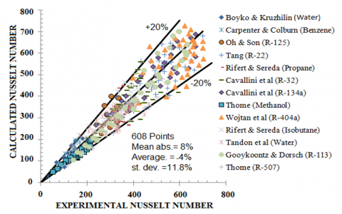
In Figure 3, the correlation between proposal model and available experimental data for horizontal tubes is shown, while, in Figure 4 a similar correlation is performed, but in this case the experimental values are correlated with the available experimental data for vertical and inclined tubes. In Figure 5 and 6 calculated (with Eqns. (77) to (79)) and experimental Nusselt are compared, the first corresponding to the vertical and inclined tubes data, while, the second is summarize horizontal tubes. In Figures 3 to 6 a 20% error bands were used.
In the models compared, only the one reported by Shah is applicable to vertical and inclined tubes, due to this situation no comparisons were made for the case of vertical and inclined tubes. However, in the study carried out, it was detected that it presents a mean deviation of 15.7%, which agrees perfectly with the original reports of the method [8], in which a mean error of 15.8% is attributed.
Table 4 summarized the mean absolute error obtained in the correlation of selected models with available experimental data [40-42].
Figure 3. Correlation of the proposal model with data for horizontal tubes
Figure 4. Correlation of the proposal model with data for vertical and inclined tubes
Figure 5. Correlation of the proposal model with data for inclined and vertical tubes
Figure 6. Correlation of the proposal model with data for horizontal tubes
Table 4. Average deviation of several models
|
Model |
EMA/H (%) |
EMA/VI (%) |
|
Shah [7, 8] |
13.9 |
15.7 |
|
Carpenter and Colburn [9] |
19.9 |
– |
|
Cavallini and Zecchin [12] |
14.6 |
– |
|
Tandon et al. [14] |
21.2 |
– |
|
Dobson and Chato [15] |
14.3 |
– |
|
Bohdal et al. [17] |
14.9 |
– |
|
Akers et al. [27] |
18.6 |
– |
|
Present work |
13.4 |
14.9 |
Note: 1. (EMA/H) is the mean deviation of horizontal tubes and (EMA/VI) is the mean deviation of vertical and inclined tubes.
A new model for heat transfer calculations in film condensation inside tubes was obtained. For this purpose, a modeling process based on FEM techniques was used, with two basic dimensionless groups being determined as guiding principles of the heat transfer process. The analysis process allows to obtain a new improved model to evaluate the heat transfer inside tubes during film condensation. This new model is valid for horizontal, vertical end inclined tubes.
The proposed model was correlated with available experimental data and it was also verified with other relationships existing in the literature, and that have been provided by other authors, detecting a better fit in the proposed model, with a mean deviation of 13.4% for horizontal tubes and 14.9% for vertical and inclined tubes.
It has been shown that the model obtained provides favorable results for flow values from 3 to 850 kg/m2s, pipe diameters from 2 to 50 mm and in the range of reduced pressures from 0.0008 to 0.91. Available data from 22 fluids were used for this purpose, including various organic compounds, water and refrigerants. In the compilation of these data, the works of a total of 33 authors of recognized prestige in the research area were consulted.
The author is very grateful for the help provided by Professor S. Thomson, from the Department of Mathematics, Massachusetts Institute of Technology, USA.
|
a |
Thermal diffusivity, m2∙s-1 |
|
B |
Konakov friction factor, used in Eq. (75) |
|
c |
Constant (0.023), used in Eq. (1) |
|
Cp |
Specific heat, J∙kg-1∙K-1 |
|
C1 |
Integration constant, defined in Eq. (34) |
|
C2 |
Integration constant, defined in Eq. (36) |
|
d |
Equivalent inner tube diameter, m |
|
D |
Constant, defined in Eq. (75) |
|
G |
Mass flux, kg∙m-2∙s-1 |
|
g |
Gravitational acceleration, m∙s-2 |
|
hfg |
Latent heat of vaporization, J∙kg-1. K-1 |
|
hfg' |
Rohsenow factor $h_{f g}^{\prime}=h_{f g}+0,375 \cdot C p_{L} \cdot\left(T_{s a t}-T_{P}\right)$ |
|
h |
Single-phase heat transfer coefficient, W∙m-2∙K-1 |
|
hT |
Two-phase heat transfer coefficient, W∙m-2∙K-1 |
|
hC |
Single-phase heat transfer coefficient, W∙m-2∙K-1 |
|
hmed |
Experimental measured value, W∙m-2∙K-1 |
|
hT |
Heat transfer coefficient determined with Eq. (70) |
|
Ja |
Jakob number |
|
Jg |
Dimensionless velocity |
|
k |
Fluid thermal conductivity, W∙m-1∙K-1 |
|
kL |
Fluid thermal conductivity for single-phase, W∙m-1∙K-1 |
|
LC |
Total length of pipe in which condensation occurred |
|
N |
Numbers of experimental points |
|
Nu |
Nusselt number |
|
NuE |
Nusselt number for experimental data |
|
NuL |
Nusselt number for single-phase used in Eq. (70) |
|
NuT |
Nusselt number for two-phase |
|
P |
Fluid pressure kg∙m-1∙s-2 |
|
PC |
Critical pressure kg∙m-1∙s-2 |
|
PrL |
Prandtl number for single-phase |
|
pR |
Reduced pressure |
|
Re |
Reynolds number |
|
Reeq |
Equivalent Reynolds number for two-phase |
|
ReL |
Liquid Reynolds number |
|
ReV |
Vapor Reynolds number |
|
T |
Mean fluid temperature, ${ }^{\circ} \mathrm{C}$ |
|
∆T |
Temperature difference across the condensate film |
|
Tsat |
Saturation temperature, ${ }^{\circ} \mathrm{C}$ |
|
TP |
Wall temperature, ${ }^{\circ} \mathrm{C}$ |
|
V |
Velocity profile, m∙s-1 |
|
VMax |
Maximum velocity, m∙s-1 |
|
Vx |
Velocity component in x axis, m∙s-1 |
|
Vy |
Velocity component in y axis, m∙s-1 |
|
Vz |
Velocity component in z axis, m∙s-1 |
|
x |
Thermodynamic vapor quality |
|
Xtt |
Dimensionless Martinelli parameter |
|
y |
Axial distance from the point where condensation started |
|
Y |
Coefficient used in Eq. (72) |
|
Z |
Dimensionless Shah parameter |
|
Greek symbols |
|
|
β |
Thermal expansion coefficient, K-1 |
|
µ |
Dynamic viscosity, kg∙m-1∙s-1 |
|
θ |
Tubes inclination respect to horizontal line |
|
ρ |
Density, kg∙m-3 |
|
ξ |
Number of intervals in function form, Eq. (20) |
|
v |
Liquid kinematic viscosity, m2∙s-1 |
|
δ |
Film thickness of boundary layer, m |
|
Φ |
Schlichting function of viscous dissipation (Eq. (4) |
|
φ |
Solution of heat transfer problem, (Eq. (12)) |
|
ψ |
Source function, (Eq. (13)) |
|
τ |
Temperature in Green’s functional, (Eq. (13)) |
|
ω |
Substituting term employed in Eq. (16) |
|
Subscripts |
|
|
L |
Liquid |
|
Superscript |
|
|
m |
Dittus-Boelter constant for $R e_{L}$ in Eq. (1) |
|
n |
Dittus-Boelter constant for $\operatorname{Pr}_{L}$ in Eq. (1) |
[1] Camaraza-Medina, Y., Rubio-Gonzales, A.M., Cruz-Fonticiella, O.M., García-Morales, O.F. (2017). Analysis of pressure influence over heat transfer coefficient on air cooled condenser. Journal Européen des Systems Automatisés, 50(3): 213-226. http://dx.doi.org/10.3166/jesa.50.213-226
[2] Boyko, L.D., Kruzhilin, G.N. (1967). Heat transfer and hydraulic resistance during condensation of steam in a horizontal tube and in a bundle of tubes. International Journal of Heat and Mass Transfer, 10(3): 361-373. https://doi.org/10.1016/0017-9310(67)90152-4
[3] Rabiee, R., Désilets, M., Proulx, P., Ariana, M., Julien, M. (2018). Determination of condensation heat transfer inside a horizontal smooth tube. International Journal of Heat and Mass Transfer, 124: 816-828. https://doi.org/10.1016/j.ijheatmasstransfer.2018.04.012
[4] Zeinelabdeen, M.I.M., Sajid-Kamran, M., Briggs, A. (2018). Comparison of empirical models with an experimental database for condensation on banks of tubes. International Journal of Heat and Mass Transfer, (122): 765-774. https://doi.org/10.1016/j.ijheatmasstransfer.2018.01.109
[5] Lee, Y.G., Jang, Y.J., Choi, D.J. (2017). An experimental study of air–steam condensation on the exterior surface of a vertical tube under natural convection conditions. International Journal of Heat and Mass Transfer, (104): 1034-1047. http://doi.org/10.1016/j.ijheatmasstransfer.2016.09.016
[6] Chen, T., Du, X., Yang, L., Yang, Y. (2015). Co-current condensation in an inclined air-cooled flat tube. Energy Procedia, 75: 3154-3161. http://doi.org/10.1016/j.egypro.2015.07.651
[7] Shah, M.M. (1979). A general correlation for heat transfer during film condensation inside pipes. International Journal of Heat and Mass Transfer, 22(4): 547-556. https://doi.org/10.1016/0017-9310(79)90058-9
[8] Shah, M.M. (2009). An improved and extended general correlation for heat transfer during condensation in plain tubes. HVAC&R RESEARCH, 15(5): 889-913.
[9] Carpenter, F.G., Colburn, A.P. (1951). The effect of vapor velocity on condensation inside tubes. In: Proceedings of the General Discussion on Heat Transfer–The Institute of Mechanical Engineers and ASME, 20-26. http://hdl.handle.net/10945/14121, accessed on April 15, 2020.
[10] Goodykoontz, J.H., Dorsch, R.G. (1966). Local heat–transfer coefficients for condensation of steam in vertical down flow within a 5/8 diameter tube. NASA Technical Reports Server. http://hdl.handle.net/2060/19660008881, accessed on April 15, 2020.
[11] Goodykoontz, J.H., Dorsch, R.G. (1967). Local heat–transfer coefficients and static pressures for condensation of high–velocity steam within a tube, NASA TND–3953. https://ntrs.nasa.gov/citations/19660008881, accessed on April 15, 2020.
[12] Cavallini, A., Zecchin, R. (1974). A dimensionless correlation for heat transfer in forced convection condensation. Proceedings Sixth International Heat Transfer Conference, Tokyo, 3: 309–313.
[13] Rosson, H.F. (1957). Heat transfer during condensation inside a horizontal tube, Ph.D. Thesis, Mechanical Engineering Department, Rice University, Houston, USA. https://scholarship.rice.edu/handle/1911/18428, accessed on April 15, 2020.
[14] Tandon, I.N., Varma, H.K., Gupta, C.P. (1995). Heat transfer during forced convection condensation inside horizontal tube. International Journal Refrigeration, 18(3): 210–214. https://doi.org/10.1016/0140-7007(95)90316-R
[15] Dobson, M.K., Chato, J.C. (1998). Condensation in smooth horizontal tubes. Journal Heat Transfer, 120(1): 193–213. http://dx.doi.org/10.1115/1.2830043
[16] Cavallini, A., Col, D.D., Doretti, L., Matkovic, M., Rossetto, L., Zilio, C., Censi, G. (2006). Condensation in horizontal smooth tubes: a new heat transfer model for heat exchanger design. Heat Transfer Engineering, 27(8): 31–38. https://doi.org/10.1080/01457630600793970
[17] Bohdal, T., Charun, H., Sikora, M. (2012). Heat transfer during condensation of refrigerants in tubular minichannels. Archives of Thermodynamics, 33(2): 3-22. http://dx.doi.org/10.2478/v10173-012-0008-x
[18] Camaraza-Medina, Y., Hernandez-Guerrero, A., Luviano-Ortiz, J.L., Cruz-Fonticiella, O.M., García-Morales, O.F. (2019). Mathematical deduction of a new model for calculation of heat transfer by condensation inside pipes. International Journal of Heat and Mass Transfer, 141: 180-190. https://doi.org/10.1016/j.ijheatmasstransfer.2019.06.076
[19] Camaraza-Medina, Y., Cruz-Fonticiella, O.M., García-Morales, O.F. (2019). New model for heat transfer calculation during fluid flow in single phase inside pipes. Thermal Science and Engineering Progress, 11: 162-166. https://doi.org/10.1016/j.tsep.2019.03.014
[20] Medina, Y.C., Khandy, N.H., Carlson, K.M., Fonticiella, O.M.C., Morales, O.F.G. (2018). Mathematical modeling of two-phase media heat transfer coefficient in air-cooled condenser systems. International Journal of Heat and Technology, 36(1): 319-324. https://doi.org/10.18280/ijht.360142
[21] Borishanskiy, V.M., Volkov, D.I., Ivashenko, N.I., Vorontsova, L.A., Illarionov, T.Y., Kretunov, O.P., Borkov, A.P., Makarova, G.A., Alekseyev, I.A. (1978). Heat transfer from steam condensing inside vertical pipes and coils. Heat Transfer Soviet Research, 10(4): 44-58.
[22] Lee, H., Yoon, J., Kim, J., Bansal, P.K. (2006). Condensing heat transfer and pressure drop characteristics of hydrocarbon refrigerants. International Journal of Heat and Mass Transfer, 49: 1922–1927. https://doi.org/10.1016/j.ijheatmasstransfer.2005.11.008
[23] Blangetti, F., Schlunder, E.U. (1979). Local heat transfer coefficients in film condensation at high Prandtl numbers. In: Marto, P.J., Kroger, P.G. (eds) Condensation Heat Transfer. ASME Press, New York.
[24] Ananiev, E.P., Boyko, L.D., Kruzhilin, G.N. (1963) Heat transfer in the presence of steam condensation in a horizontal tube. International Developments in Heat Transfer, Proceedings of 1961-62 Heat Transfer Conference, Boulder, Colorado and London, Part 2, pp. 290-295.
[25] Tepe, J.B., Mueller, A.C. (1947). Condensation and subcooling inside an inclined tube. Chemical Engineering Progress, 43(5): 267- 278.
[26] Yan, Y., Lin, T. (1999). Condensation heat transfer and pressure drop of refrigerant R-134a in a small pipe. International Journal of Heat and Mass Transfer, 42: 697–708. https://doi.org/10.1016/S0017-9310(98)00195
[27] Akers, W.W., Deans, H.A., Crosser, O.K. (1959). Condensing heat transfer within horizontal tubes. Chemical Engineering Progress Symposium Series, 55(29): 171-176.
[28] Lemmon, E., Huber, M., McLinden, M. (2013). NIST Standard Reference Database 23: Reference Fluid Thermodynamic and Transport Properties-REFPROP, Version 9.1, Natl Std. Ref. Data Series (NIST NSRDS), National Institute of Standards and Technology, Gaithersburg, MD. https://tsapps.nist.gov/publication/get_pdf.cfm?pub_id=912382.
[29] Tang, C.C. (2011). A study of heat transfer in non-boiling two-phase gas-liquid flow in tubes for horizontal, slightly inclined, and vertical orientations. Ph.D. Thesis. Mechanical Engineering Department, Oklahoma State University, Stillwater, Oklahoma, USA.
[30] Mollamahmutoglu, M. (2012). Study of isothermal pressure drop and non-boiling heat transfer in vertical downward two-phase flow, MSc. Thesis. Mechanical Engineering Department. Oklahoma State University, Stillwater, Oklahoma, USA.
[31] Cavallini, A., Censi, G., Del Col, D., Doretti, l., Longo, G.A., Rossetto, l., Zilio, C. (2003). Condensation inside and outside smooth and enhanced tubes – a review of recent research. International Journal of Refrigeration, 26(4): 373–392. http://dx.doi.org/10.1016/S0140-7007(02)00150-0
[32] Oh, H.K., Son, C.H. (2011). Condensation heat transfer characteristics of R-22, R-134a and R-410A in a single circular microtube. Experimental Thermal Fluid Sciences, 35(4): 706-716. https://doi.org/10.1016/j.expthermflusci.2011.01.005
[33] Wojtan, l., Ursenbacher, T., Thome, J.R. (2005). Investigation of flow boiling in horizontal tubes: Part II. Development of a new heat transfer model for stratified-wavy, dry out and mist flow regimes. International Journal of Heat and Mass Transfer, 48(14): 2970–2985. https://doi.org/10.1016/j.ijheatmasstransfer.2004.12.013
[34] Rifert, V.G., Sereda, V.V., Barabash, P.O., Gorin, V.V. (2017). Condensation inside Smooth Horizontal Tubes: Part 2. Improvement of Heat Exchange Prediction. Thermal Science, 21(3): 1479-1489. https://doi.org/10.2298/TSCI140815045R
[35] Thome, J.R. (2005). Condensation in plain horizontal tubes: recent advances in modelling of heat transfer to pure fluids and mixtures. Journal of the Brazilian Society of Mechanical Sciences and Engineering, 27(1): 23-30. http://dx.doi.org/10.1590/S1678-58782005000100002
[36] Cttani, L., Bozzoli, F., Raineri, S. (2017). Experimental study of the transitional flow regime in coiled tubes by the estimation of local convective heat transfer coefficient. International Journal of Heat and Mass Transfer, 112: 825-836. https://doi.org/10.1016/j.ijheatmasstransfer.2017.05.003
[37] Ali, H. M., Qasim, M. Z., Ali, M. (2016). Free convection condensation heat transfer of steam on horizontal square wire wrapped tube. International Journal of Heat and Mass Transfer, 98: 350-358. https://doi.org/10.1016/j.ijheatmasstransfer.2016.03.053
[38] Ali, H.M. (2017). An analytical model for prediction of condensate flooding on horizontal pin-fin tubes. International Journal of Heat and Mass Transfer, 106: 1120-1124. https://doi.org/10.1016/j.ijheatmasstransfer.2016.10.088
[39] Camaraza-Medina, Y., Hernández-Guerrero, A., Luviano-Ortiz, J.L., Mortensen-Carlson, K., Cruz-Fonticiella, O.M., García-Morales, O.F. (2019). New model for heat transfer calculation during film condensation inside pipes. Int. J. Heat Mass Transfer, 128, 344-353. https://doi.org/10.1016/j.ijheatmasstransfer.2018.09.012
[40] Camaraza-Medina, Y., Sanchez-Escalona, A.A., Cruz-Fonticiella, O.M., García-Morales, O.F. (2019). Method for heat transfer calculation on fluid flow in single-phase inside rough pipes, Thermal Science and Engineering Progress, 14: 100436. https://doi.org/10.1016/j.tsep.2019.100436
[41] Rifert, V., Sereda, V., Gorin, V., Barabash, P., Solomakha, A. (2020). Heat transfer during film condensation inside plain tubes. Heat Mass Transfer, 56: 691-713. https://doi.org/10.1007/s00231-019-02744-5
[42] Camaraza-Medina, Y., Hernandez-Guerrero, A. Luviano-Ortiz, J.L. (2020). Comparative study on heat transfer calculation in transition and turbulent flow regime inside tubes, Latin American Applied Research, 50(4): 309-314. https://doi.org/10.52292/j.laar.2020.580