Gennadiy A. Gorbenko | Pavlo G. Gakal | Rustem Yu. Turna | Artem M. Hodunov | Edem R. Reshytov*
© 2021 IIETA. This article is published by IIETA and is licensed under the CC BY 4.0 license (http://creativecommons.org/licenses/by/4.0/).
OPEN ACCESS
The paper proposes a model of heat transfer in the evaporator of the spacecraft thermal control system. The model allows to calculate the average temperature of the evaporator wall and to build a "boiling curve" in a wide range of thermal loads.
Adequacy of the model is confirmed by experimental studies on an aluminum thermal sink with high longitudinal thermal conductivity in the range of parameters typical for the thermal control systems of spacecrafts. Ammonia is used as a working fluid. The model might be recommended for use in zero gravity and normal ground conditions.
average heat-transfer coefficient, ammonia, boiling curve, evaporator, mechanically pumped two-phase loop, subcooled boiling, saturated boiling, two-phase thermal control system
One of the most important tasks of spacecraft design is providing their thermal regime. Currently, there is a tendency to use in spacecraft with heat generation over 5 kW thermal control systems (TCS) based on mechanically pumped two-phase loops (MPTL) [1-3].
MPTL have several advantages over single-phase thermal control systems. In particular, MPTL can transfer much more heat per unit of mass flow rate than with single-phase heat transfer systems. Energy consumption of pump for working fluid pumping is low. Heat transfer by means of boiling allows maintaining temperature of objects at almost entire length of the loop close to saturation temperature. Heat transfer processes where aggregate state of substance changes take place (boiling, condensing) are much more intense than those where convective heat transfer in a single-phase liquid occurs. These features of MPTL result in a significantly lower mass of thermal control system compared to single-phase system. Therefore, the task of creating TCS on the basis of MPTL is actively solved all over the world. For example, this task is included in the program of NASA prospective works [4] for 2015-2035.
The main element of MPTL heat acquisition subsystem is a thermal sink - a contact heat exchanger, on surface of which the cooled components are fixed. The heat from components is drawn to the thermal sink and then to the thermal fluid, which is pumped through the channel evaporator. There is a section of "subcooled boiling" in case of subcooled liquid at evaporator inlet, where heat is transferred by surface boiling of fluid. At present, however, the calculation of thermal sinks for both space and ground applications has not been sufficiently worked out. Particularly this is the case of thermal sink, where subcooled single-phase liquid at inlet and two-phase flow at outlet. In this case, depending on heat flux density and parameters of working fluid, there may be a section of "subcooled boiling" - a section where the heat transfer takes place due to surface boiling in subcooled liquid.
The research aims to develop a model for calculating heat transfer and average evaporator wall temperature in presence of subcooled boiling section in a wide range of parameters specific for thermal control systems of space vehicles. In particular:
- ammonia saturation temperature - from sub-zero temperatures to +75℃;
- liquid ammonia subcooling at the evaporator inlet - from 0 to 30 K;
- mass velocity - from 27 to 200 kg/(s*m2);
- average heat flux density on the evaporator wall - from 0 to 18 W/cm2.
Problems of heat transfer at forced convection [5, 6] and saturated boiling in channels [7-9] are well investigated, numerous correlations and methods are developed for calculation of local heat transfer coefficients and evaporator wall temperature. However, calculating the heat transfer during surface boiling in subcooled liquid still have certain difficulties at present. Performed experimental research is mainly related to boiling of water. Data on ammonia boiling are limited [10]. To determine the heat transfer intensity in the section of subcooled boiling it is necessary to perform additional experimental studies in the range of parameters specific for spacecraft thermal control system.
Figure 1 shows the modern outlooks of heat transfer mechanism of liquid in uniformly heated channel in a presence of subcooled boiling [11].
Heat transfer in zone A is determined by forced convection of liquid. The convective heat transfer coefficient of liquid is almost constant (without an account of properties change with temperature), wall temperature increases linearly and parallel to liquid temperature. The first bubbles appear on the wall at ONB point (beginning of zone B), which is identified as beginning of surface boiling. There is usually a temperature jump associated with a sharp increase in heat transfer intensity in this cross-section. The contribution of boiling to heat transfer is higher with flow downstream following, while the single-phase convective heat transfer contribution decreases. It's a partial subcooled boiling interval. At the FDB point the convective contribution to the total heat transfer becomes insignificant and a fully developed subcooled boiling is established (zone C1). Following on the flow, the average temperature of liquid reaches saturation temperature and developed boiling take place in already saturated liquid (zone С2). The wall temperature remains almost constant in zones С1 and С2.
Figure 1. Distribution of wall and liquid temperature, mass vapor quality along the length of a uniformly heated channel
In contrast to free convection (Pool boiling), forced convection affects the heat transfer in addition to the boiling heat transfer when liquid flow in the channel [12, 13]. The combined effect of these two mechanisms of heat transfer takes place in all regions of the heated channel: subcooled boiling and boiling in saturated liquid. The contribution of forced convection to the total heat transfer is mainly determined by the flow rate: it could be close to zero or almost completely determines the heat transfer intensity. In the subcooled boiling section, these two mechanisms are always compatible: at the beginning of the section, the heat transfer is fully determined by convection, at the end of the section, the boiling contribution becomes the determining factor [14, 15].
Numerous experiments show that in channels at developed subcooled boiling or boiling in saturated liquid up to the volume vapor quality of the flow ~ 0.7 the contribution of the convective component can usually be neglected [5]. The heat transfer coefficient in this section does not depend either on subcooling or on the mass flow rate of the working fluid. It can be calculated as a developed saturated boiling (Pool boiling) [16, 17].
Various models have been proposed to calculate the heat transfer for the forced flow where the boiling take place. The paper [18] provides a review of the most common models. In all models, the flow region is divided into characteristic heat transfer zones: single-phase convection, subcooled boiling and developed boiling. The boundaries of each area are set differently in different models. Calculation of heat transfer in the zone of subcooled boiling is based on the superposition principle. For example, in Labuntsov model [5], the whole range of possible values of heat transfer coefficients is divided into three zones distinguished by different contribution of heat transfer convective component. In this case dimensionless coordinates are used hq/hL.
The author identifies the following zones:
In zone 1, hq/hL <0.5, hTP = hL – boiling does not affect heat transfer. The heat transfer intensity is fully determined by the forced convection of the liquid.
In zone 2, hq/hL> 2, hTP = hq – the heat transfer intensity is completely determined by developed pool boiling; forced convection does not affect heat transfer.
In zone 3, 0.5 ≤ hq/hL ≤ 2 – transient boiling zone with the mutual influence of convective heat transfer and boiling heat transfer; the expression for the heat transfer coefficient is described by the interpolation formula:
$h_{T P}=h_{L} \cdot\left(4 \cdot h_{L}+h_{\varphi}\right) /\left(5 \cdot h_{L}+h_{q}\right)$ (1)
Also note that most models [8, 19] consider local heat transfer coefficients and wall temperatures along the length of a uniformly heated channel. However, in engineering tasks of thermal state calculation of thermal sink, especially thermal sink with high longitudinal thermal conductivity, it is of interest not to describe in detail the wall temperature changes along the length of the heated channel, but to determine the average or maximum wall temperature of the heat transfer device. For this purpose, it is rational to use the concept of average heat transfer coefficient along the perimeter and length of evaporator and the simple ratios for calculation of average wall temperature Tw.
The paper proposes a model for calculating the average wall temperature of a thermal sink with large longitudinal thermal conductivity. The model makes it possible to calculate the intensity of heat transfer in each zone. At the same time, the boundaries of each zone are justified experimentally for the parameters, typical for TCS of spacecrafts. Ammonia is used as a working fluid. Adequacy of the model is confirmed by experimental results.
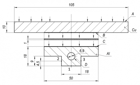
The experimental model of the thermal sink (Figure 2) consists of two parts: a copper plate and an aluminum alloy profile. An electric heater is installed on the "A" surface of the copper plate (not shown in the Figure 2), which uniformly supplies heat over the entire surface. The heat is transferred from the copper plate to the aluminum profile through the surfaces "B" and "C", through a gasket of graphite layer 1 mm thick. Thermal resistance of the graphite layer (including two contact resistances) is R = 0.000435 (m²·K)/W. Then heat flows through the surface "D" from the aluminum profile to the ammonia, which is flowing through a cylindrical channel with a diameter of 6.9 mm and a length of 150 mm. The heat transfer surface area of the channel Fev =32.5 сm². Roughness of the heat transfer surface of the channel (surface "D"):
Ra = 3.33 µm, Rz = 26.89 µm. Thermal conductivity of the profile material 180 W/(m∙K). Thermal conductivity of copper plate 392 W/(m∙K).
Aluminum profile temperatures were measured by PT-1000 type resistance sensors in three cross-sections along profile length: in the middle of the thermal sink and at a distance of 37.5 mm from the beginning and end. There are three sensors installed on each profile section at points 1, 2 and 3 (Figure 2). A total of 9 temperature sensors are installed on the surface of profile.
Figure 2. Cross section profile of the experimental thermal sink
Ammonia with a given pressure, mass flow rate and temperature were supplied to the thermal sink inlet in experiment.
The experiments are performed in the following range of parameters:
• saturation temperature Tsat = 35 … 75℃;
• inlet fluid subcooling ∆Tsub = 0…30℃;
• mass flow rate m = 0.2…7.5 g/s;
• mass velocity: G = 5…200 kg/(s*m2);
• average heat flux density q = 0…18 W/cm2.
The experiments are performed in three thermal sink orientation: two horizontal (heater installed at the top or bottom) and one vertical (upstream).
The parameters were measured in the experiments:
• inlet pressure of the thermal sink рHCA;
• mass flow rate m;
• heater power Q;
• inlet and outlet thermal sink temperatures Tin, Tex;
• temperatures on thermal sink surface (9 sensors) Tw1...Tw9.
Instrumental measurement errors of parameters:
- absolute pressure ± 0.2 %;
- mass flow rate of liquid ± 0.2%;
- temperature: ± 0.15°C (0℃), ± 0.35℃ (100℃).
To avoid heat loss, the thermal sink was insulated. Heat loss was not more than 3% and was not taken into account under the analysis of results.
The thermal state of the thermal sink was analyzed using SolidWorks Flow Simulation tool for different heater powers. The analysis showed that in the fixed cross-section of the thermal sink the average surface temperature D is almost equal to the average measured temperature of three sensors installed in points 1, 2, 3 on the profile surface (Figure 2). At the same time, the analysis showed high longitudinal heat conductivity of the structure: the average temperature difference in three cross-sections did not exceed 1K. Therefore, the average temperature of the heat transfer surface along the perimeter and length of the Tw evaporator was determined by averaging the readings of 9 sensors on the profile of the thermal sink. With that, the methodological error is about 1K.
Based on measured results next parameters were calculated:
• average heat flux density over surface "D":
$q=Q / F_{\text {ev }}, \mathrm{W} / \mathrm{cm}^{2}$; (2)
• saturation temperature Tsat as a function of pressure;
• liquid subcooling at the evaporator inlet ∆Тsub:
$\Delta T_{\text {suk }}=T_{\text {sat }}-T_{\text {in }}, \mathrm{K}$; (3)
• vapor quality хex at the evaporator outlet:
$x_{e x}=\left(Q / m-C_{p} \cdot \Delta T_{s u b}\right) / r$, (4)
where, Cp – is heat capacity at constant pressure of the liquid working fluid, J/kg/K, r – latent heat of vaporization, J/kg.
If the balance vapor quality хex was negative, the balance temperature of liquid at the outlet channel was also calculated:
$T_{e x . b}=T_{i n}+Q /\left(C_{p} \cdot m\right)$ (5)
The heat transfer equation was used to find an effective average heat transfer coefficient $\mathrm{h}_{\mathrm{ef}}$. In this case, the effective average temperature of working fluid was specially indicated $\mathrm{T}_{\mathrm{ef}}$:
$h_{e f}=q /\left(T_{w}-T_{e f}\right)$ (6)
The main results relate to the horizontal orientation of thermal sink "heater on top". Comparison with experiments in other orientations of thermal sink (vertical and horizontal "heater at the bottom") has shown that in the horizontal "heater at the top" orientation we get the most conservative result, the highest Tw values in similar modes. The difference in Tw value in the range of the performed experiments did not exceed 1...2 K and appeared only at low mass flow rates of the working fluid, less than 1 g/s (mass velocity less than 27 kg/(s*m2)). Thus, it is determined that at higher flow rates the influence of gravity is insignificant and the results obtained can be used for conditions of zero gravity.
The experimental results are presented as "boiling curves". Instead of traditional representation of a "boiling curve" in coordinates q = f(Tw), the dependence Tw = f(q) is used.
In Figure 3 one of characteristic dependencies is considered in detail. It can be seen that with q increasing the average wall temperature Tw increases with a constant value of saturation temperature Tsat, flow rate m, and liquid subcooling at the inlet ∆Тsub. The same figure shows the change in mass vapor quality хex at the outlet of thermal sink. Negative values of хex don't have physical sense, but show the degree of subcooling of the flow at the outlet of the thermal sink.
Analysis of dependencies Tw = f(q) allowed to allocate three zones with different character of temperature change:
- Zone "A" - zone of heat transfer during single-phase fluid convection. Wall temperature below the saturation temperature.
- Zone "C" - zone of developed saturated boiling. Wall temperature above saturation temperature. Slight increase in wall temperature with a significant increase in specific heat flux.
- Zone "B" - transition zone of subcooled boiling. Wall temperature above the saturation temperature.
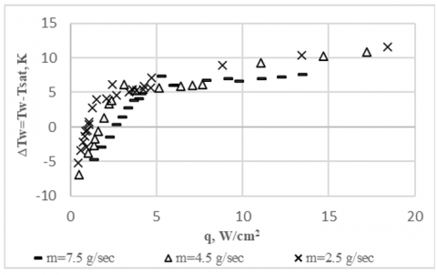
In Figures 4-6 shows other experimental dependencies of wall overheating ∆Tw = Tw - Tsat on average heat flux density q. On a basis of the results obtained it is possible to analyze the influence of mass flow, saturation temperature and liquid subcooling at the inlet on the wall temperature Tw.
Figure 3. Experimental dependence Tw = f(q). (Tsat = 55℃; m = 7.5 g/s; ΔTsub = 10 K)
As shown in Figure 4, the mass flow rate only affects the position of zones "A" and "B" and almost don’t have impact to the overheating of the wall temperature at high heat fluxes in zone "C".
Figure 4. Dependence of wall temperature overheating ∆Tw on heat flux density q at different mass flows m (Tsat = 55℃, ΔTsub = 10 K)
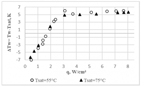
Figure 5. Dependence of wall temperature ∆Tw overheating on heat flux density q at different saturation temperatures (m = 4.5 g/s, ΔTsub = 10 K)
Figure 5 shows experimental dependencies of overheating of wall temperature ∆Tw on specific heat flux density q at different saturation temperature Tsat. It can be seen that the change of saturation temperature from 55℃ to 75℃ does not affect the slope of the curve in zone "A". In zone "C" overheating of the wall slightly decreases with increasing saturation temperature from 55℃ to 75℃, that corresponds to increasing pressure from 23.1 to 37.1 bar.
Figure 6 shows experimental dependencies of overheating of wall temperature ∆Tw on average heat flux density q at different liquid subcooling of working fluid ∆Tsub at evaporator inlet. It can be concluded that subcooling affects the position of zones "A" and "B", but the wall temperature Tw at high heat fluxes density in zone "C" subcooling has not significantly impacted.
Figure 6. Dependence of wall temperature ∆Tw overheating on heat flux density q with different subcooling at the inlet (Tsat = 75℃, m = 7.5 g/s)
This behavior of the dependencies ∆Tw=f(q) in the range of the conducted experiments allows us to state that:
- in the zone "A" the heat transfer is determined mainly by the liquid convection with a constant heat transfer coefficient. The boiling heat transfer contribution is very small or absent. The zone "A" can be limited by condition Tw = Tsat.
- in zone "C" heat transfer is independent of liquid subcooling and mass flow rate and is determined mainly by the specific heat flux;
- zone "B" is characterized by a smooth change of derivative dTw/dq from zone "A" to zone "C". In this zone, the contribution of convective heat transfer and boiling is commensurable.
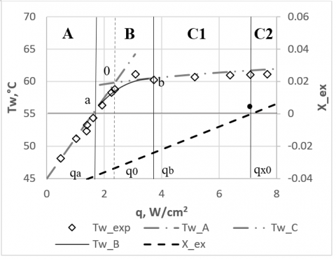
The heat transfer model in evaporator of thermal sink for specific heat flux density q varies from zero to the maximum value, which correspond to the developed saturated boiling mode, is given below.
The model is illustrated in Figure 7. The full range of heat transfer in the thermal sink evaporator Tw=f(q) s divided into three zones: А, В, С. There are calculated boiling curve and heat transfer zones are applied on the experimental results on figure. The calculated balance vapor quality xex is also given. As can be seen, there is a liquid at thermal sink outlet up to qx0 ≈ 7.1 W/m2. The section of the boiling curve from qa to qx0 can be conventionally called as section of "subcooled boiling".
Figure 7. Heat transfer zones
The model includes determination of boundaries of zones A, B, C, effective average temperature value of working fluid Tef and sequential computation of heat transfer in each zone (calculation of Tw and hef).
As input data for model are specified:
• Tsat – saturation temperature in thermal sink evaporator, ℃;
• ∆Tsub – liquid subcooling at the evaporator inlet, К;
• m – mass flow rate, kg/s;
• Fev – evaporator heat transfer surface, m2;
• d,L− diameter and length of the evaporator, m;
• Q – thermal sink heat load, W.
Calculated parameters:
• Tw – average heat transfer surface temperature, ℃;
• Tef – effective average temperature of the working fluid, ℃;
• hef – calculated heat transfer coefficient, W/(m²·K);
• хex – mass vapor quality at the evaporator outlet.
• average heat flux density q (Eq. (2)), W/m2;
• evaporator inlet temperature Tin (Eq. (3)), ℃;
• evaporator outlet temperature Tex (Eq. (5)), ℃.
Hereinafter, the index "calc" was omitted.
Note: calculation from the given input data allows to determine only Tw and хex. To find the heat transfer coefficient hef according to the Eq. (6), you first need to determine the effective temperature of the coolant Tef. In different zones of the boiling curve, it is determined in different ways.
Since it is not possible to determine the heat transfer zone at once at a given value Q, a sequential calculation of boundaries and heat transfer in all three zones of the boiling curve is implemented.
Zone A - convective single-phase heat transfer, linear dependence Tw = f(q)
The calculation is performed according to traditional methods for heat transfer of single-phase liquid in channels [20, 21]. If some simplifying assumptions are accepted, then can be written down:
• effective average temperature of the working fluid:
$T_{\text {ef. } A}=\left(T_{\text {in }}+T_{\text {ex }}\right) / 2=T_{\text {in }}+\left(q \cdot F_{\text {ev }}\right) /\left(2 \cdot C_{p} \cdot m\right)$ (7)
• thermophysical properties of a liquid are considered as constant and correspond to Тef.А;
• heat transfer coefficient: $\mathrm{h}_{\mathrm{L}, \mathrm{A}}=\mathrm{Nu} \cdot \lambda_{\mathrm{L}} / \mathrm{d}$, where Nu is determined according to the flow pattern by known correlations for single-phase flow [20, 21];
the average wall temperature in zone "A" can be determined from the equation:
$T_{w \cdot A}=T_{i n}+q \cdot\left(F_{e v} /\left(2 \cdot C_{p} \cdot m\right)+1 / h_{L}\right)$ (8)
Essentially, this equation is a straight line Тw = f(q), as the heat transfer coefficient in this zone changes slightly, what is confirmed by the experiment.
The boundary of zone "A" is defined from the condition: Tw.a = Tsat.
At the border (at point "a"):
$T_{w \cdot a}=T_{\text {sat }}$. (9)
$q_{a}=\left(T_{w . a}-T_{i n}\right) /\left(F_{e x} /\left(2 \cdot C_{p} \cdot m\right)+1 / h_{L, A}\right)$ (10)
Zone C - developed boiling zone (С1 - in subcooled liquid; С2 – in saturated liquid)
The effective heat transfer coefficient in zone C can be calculated by correlations for developed boiling in channels with correction for flow velocity (mass flow rate) [9]. The influence of flow velocity on heat transfer in this zone up to the volume vapor content at the outlet ~ 0.8 cannot be taken into account and it is acceptable to use heat transfer coefficients for pool boiling.
The heat transfer coefficient for pool boiling is proposed to be calculated by Kupriyanova formula [10].
$h_{e f . C}=h_{q \cdot C}=2.2 \cdot p^{0.21} \cdot q^{0.7}$ (11)
In spite of the fact that this correlation was obtained for boiling on the surface of a horizontal tube in the temperature range from -40…+20℃, and our experiments were carried out in the temperature range of +35...+75℃, comparison with the experiment showed that the formula quite well describes all performed series of experiments. The difference between experimental and calculated Tw, values did not exceed 2 K.
The effective temperature in zone "C" is:
$T_{e f . C}=T_{\text {sat }}$ (12)
The average wall temperature in zone C at any heat flux density is determined from the heat transfer equation (Eq. (6)):
$T_{w . C}=T_{\text {ef.C }}+q / h_{\text {ef.C }}$ (13)
The top border of zone C qmax is limited by volume vapor quality ~ 0.7...0.8. Nevertheless, as experimental results show, satisfactory matching of the theory and experiment was observed up to хex ≈ 0.7…0.8.
The lower boundary of the zone qb is determined by the algorithm below.
Zone B - transition zone of subcooled boiling in part of evaporator channel
The boundaries of zone "B" are indicated by points "a" and "b" on the boiling curve. The parameters in this zone change smoothly without jumps and curve breaks from point "a" to point "b". Therefore, to describe the function Tw =f(q) in the zone "B", it is acceptable to use approximation in the form of a Bezier spline function [22] without derivative discontinuity in the points "a" and "b".
Note: Some outliers of experimental values Tw in zone B (Fig. 3 and 7) are explained by different number of active centers of steam formation on the heat-exchange surface at increase and decrease of specific heat flux. This phenomenon is known and called "heat flux hysteresis" [10]. In experiments with aluminum thermal sink, the hysteresis was small. However, in stainless steel smooth channels for ammonia heat transfer, the hysteresis can be more than 10K.Therefore, our proposed methodology for calculating the parameters in the transition zone B refers to the process of reducing the heat load from the developed boiling zone, when most of the vaporization centers are activated.
The tangents in the points "a" and "b" should be drawn up to theirs intersect at point "0" in order to trace the Bezier curve. By the three points "a", "b" and "0" the Bezier function (Figure 7, line Tw.b) could be found. Thus, to find the function Tw =f(q) in the zone B, the coordinates of the points "a", "b" and "0" should be available.
The coordinates of point "a" are determined according to Eq. (9) and (10).
To determine the width of the transition zone "B" and the coordinates of point "b" we use Labuntsov approach - use dimensionless coordinates hq/hL [5].
Determine the position of points "a", "0" and "b" relative to each other in coordinates hq/hL.
The difference in the "a" and "0" points position in the non-dimensional coordinates is equal:
$\Delta\left(h_{q} / h L\right)_{a-0}=\left(h_{q} / h_{L}\right)_{0}-\left(h_{q} / h_{L}\right)_{a}$ (14)
We will estimate the position of point "0" by the results of experimental studies. It is determined that $\Delta\left(\mathrm{h}_{\mathrm{q}} / \mathrm{h}_{\mathrm{L}}\right)_{\mathrm{a}-0}$ changes depending on parameters of the working fluid at the thermal sink inlet in very insignificant limits, from 0.65 to 0.70.
Since the curve Tw.q=f(q) in the area of point "b" is slightly sloping, its location can be assigned approximately by taking the offset of points "a" and "b" in dimensionless coordinates:
$\Delta\left(h_{q} / h_{L}\right)_{a-b} \approx 2 \Delta\left(h_{q} / h_{L}\right)_{a-0} \approx 1.5$ (15)
$\left(h_{q} / h_{L}\right)_{b}=\left(h_{q} / h_{L}\right)_{a}+1.5$ (16)
The further algorithm for calculating the coordinates of point "b" is as follows:
- determine the heat transfer coefficient in point "a" hLа by known correlations for single-phase flow;
- knowing the heat flux density qa at point "a" (Eq. (10)), the heat transfer coefficient at boiling hqa should be calculated by the Eq. (11).
- find a dimensionless relation $\left(\mathrm{h}_{\mathrm{q}} / \mathrm{h}_{\mathrm{L}}\right)_{\mathrm{a}}$ at point "a";
- calculate a dimensionless relation $\left(\mathrm{h}_{\mathrm{q}} / \mathrm{h}_{\mathrm{L}}\right)_{\mathrm{b}}$ at the point "b" by the Eq. (16);
- determine the heat transfer coefficient of boiling at the point "b" considering that $\mathrm{h}_{\mathrm{L.b}} \approx \mathrm{h}_{\mathrm{L.a}}$:
$h_{q . b}=h_{L . b} \cdot\left(h_{q} / h_{L}\right)_{b}$ (17)
- calculate the heat flux density at point "b" by transforming the Eq. (11):
$q_{h}=\left(h_{q, b} / 2 \cdot 2 \cdot p^{0.21}\right)^{\frac{1}{0.7}}$ (18)
- wall temperature at this point:
$T_{w \cdot b}=T_{s a t}+q_{h} / h_{q . b}$ (19)
Find the derivatives at points "a" and "b": $\alpha=\left(d T_{w . A} / d q\right)_{a}=F_{e v} /\left(2 \cdot C_{p} \cdot m\right)+1 / h_{L}$ (see. Eq. (8));
$\beta=\left(d T_{w . C} / d q\right)_{b}=0.3 / h_{q . b}$ (see. Eq. (13)).
The coordinates of the point "0" should be found as intersection of tangents:
- heat flux density at point "0":
$q_{0}=q_{a}+\left[\left(T_{w . b}-T_{s a t}\right)-\left(q_{b}-q_{a}\right) \cdot \beta\right] /(\alpha-\beta)$
- wall temperature at point "0":
$T_{w .0}=T_{s a t}+\left(\left[\left(T_{w . b}-T_{s a t}\right)-\left(q_{b}-q_{a}\right) \cdot \beta\right] /(\alpha-\beta)\right) \cdot \alpha$
Having coordinates of three points "a", "b" and "0" the Bezier quadratic curve could be drawn [22], by which we determine the temperature of the wall in any point of zone B.
The heat transfer coefficient in zone "B" does not make sense to find, because it is not defined how the Tef value in this zone changes.
The paper presents the heat transfer model in evaporator of thermal sink of heat acquisition thermal control subsystem. The method allows determining the average evaporator wall temperature in a wide range of heat loads, mass velocities, saturation temperatures, liquid subcooling at the inlet. Saturated or subcooled liquid can enter the evaporator. The model is valid for thermal sinks with large longitudinal thermal conductivity when the wall temperature along the evaporator changes only slightly.
The model takes into account different modes of heat transfer: single-phase convective heat transfer of liquid; transitional zone of "partial subcooled boiling"; zone of "developed boiling" in subcooled or saturated liquid. For each mode, the heat transfer is calculated using a different method.
The computational model has been tested in experiments on a thermal sink with an aluminum evaporator and ammonia as a working fluid in the range of parameters typical for two-phase thermal control systems of space vehicles. Three characteristic heat transfer zones are considered.
Zone "A" (single-phase convection). Heat transfer is calculated according to generally accepted methods for single-phase liquid flow in channels. The wall temperature is below the liquid saturation temperature. Average logarithmic (or medium-arithmic) temperature head is used in heat transfer equation.
Zone "B" (transition zone of subcooled boiling), to which the contribution of boiling and convection are comparable. The wall temperature is above the saturation temperature. The model suggests calculating the average wall temperature directly, using a Bezier spline function to approximate the wall temperature between zones "A" and "C".
Zone "C" (developed boiling). The heat transfer coefficient is calculated using the formulas for developed boiling. The temperature head is equal to the difference between the surface temperature and the saturation temperature.
The proposed method can be used for thermal sinks of any length. The experimental thermal sink had a length of 150 mm and high longitudinal thermal conductivity, which provided a uniform wall temperature over the entire length of the evaporator. Obviously, there are no concerns associated with shorter length thermal sinks. In limit case (L à0) the model will be transformed to the traditional method of local parameters calculating in the channel.
To analyze the applicability of model to microgravity conditions, experiments were performed with different orientation of thermal sinks: horizontal (heater at the top or bottom of the channel) and vertical (upward flow). It is determined that at a mass velocity above 27 kg/(s*m2) the influence of orientation and location of the heater on the intensity of heat transfer is insignificant, the difference in wall temperature does not exceed 1...2 K. Therefore, the method can be recommended for microgravity conditions as well.
|
p |
pressure, bar |
|
T |
temperature, °C, K |
|
ΔT |
temperature difference, |
|
m |
mass flow rate, gm/s, kg/s |
|
Q |
heat load, W |
|
q |
heat flux density, W/m2 |
|
F |
surface area, m2 |
|
d |
diameter, m |
|
L |
length, m |
|
h |
heat transfer coefficient, W/(m2∙K) |
|
Re |
Reynolds number |
|
Pr |
Prandtl number |
|
Cp |
heat capacity at constant pressure, J/(kg∙K) |
|
G |
mass velocity, kg/(s*m²) |
|
x |
vapor quality, kgv/kgf |
|
Nu |
Nusselt number |
|
R |
thermal resistivity, (m² ·K)/W |
|
Greek symbols |
|
|
ρ |
density, m3/kg |
|
λ |
thermal conductivity, W/(m∙K) |
|
µ |
dynamic viscosity, kg. m-1.s-1 |
|
Subscripts |
|
|
A |
Zone "A" |
|
B |
Zone "B" |
|
C |
Zone "C" |
|
a |
point "a" |
|
b |
point "b |
|
w |
wall |
|
q |
developed boiling |
|
ef |
effective |
|
calc |
calculation parameter |
|
TP |
target value of heat transfer coefficient |
|
L |
single-phase liquid |
|
v |
vapor |
|
ev |
evaporator |
|
in |
inlet |
|
ex |
exit |
|
sat |
saturation |
|
sub |
subcooling |
|
ONB |
Onset of Nucleate Boiling |
|
FDB |
Fully Developed Boiling |
[1] Gorbenko, G.A., Prokhorov, Y.M., Cykhotsky, V.M. (1997). Designing problems of two-phase central thermal control system for the International Space Station. Sixth European Symposium on Space Environmental Control Systems, held in Noordwijk, The Netherlands, 20-22 May. Compiled by T.-D. Guyenne. European Space Agency, SP-400, pp. 439.
[2] Hugon, J., Delmas, A., Gakal, P.G., Gorbenko, G.A., Turna, R., Chayka, D.V. (2016). Heat transfer in finned evaporator channels of two-phase thermal control system for microgravity conditions. 46th International Conference on Environmental Systems, Vienna, Austria.
[3] Basov, A.A., Leksin, M.A., Prokhorov, Y.M. (2017). A Two-phase loop of thermal control system of science-power module. Numerical simulation of hydraulic characteristics. S.P. Korolev Rocket and Space Public Corporation Energia (in Russian). https://readera.org/14343558
[4] Hill, S.A., Kostyk, C., Moril, B., Notardonato, W., Rickman, S., Swanson, T. (2012). NASA technology roadmaps, TA 14: Thermal management systems. National Aeronautics and Space Administration, Washington, DC. https://www.nasa.gov/sites/default/files/atoms/files/2015_nasa_technology_roadmaps_ta_14_thermal_management_final.pdf.
[5] Labuntsov, D. (2000). Physical fundamentals of power engineering. Selected works on heat transfer, fluid mechanics and thermodynamics. M.: MPEI, 2000 (in Russian).
[6] Winterton, Z.L. (1991). A general correlation for saturated and subcooled flow boiling in tubes and annuli, based on a nucleate pool boiling equation. Int. J. Heat Mass Transfer, 34(11): 2759-2766. https://doi.org/10.1016/0017-9310(91)90234-6
[7] Chen, J.C. (1963). A correlation for boiling heat transfer to saturated fluids in convective flow. Proceeding of 6th National Heat Transfer Conference, Boston, USA. https://doi.org/10.1021/i260019a023
[8] Bowring, R.W. (1962). Physical model based on bubble detachment and calculation of steam voidage in the subcooled region of a heated channel. HPR-10, Institute for Atomenergi, Halden, Norway.
[9] Kandlikar, S.G. (1990). A general correlation for saturated two-phase flow boiling heat transfer inside horizontal and vertical tubes. ASME Journal of Heat Transfer, 112(1): 219-228. https://doi.org/10.1115/1.2910348
[10] Kupriyanova, A.V. (1970). Heat transfer at ammonia boiling on the horizontal pipes (in Russian) / A.V. Kupriyanova, 11: 40-44.
[11] Collier, J.G., Thome, J.R. (1994). Convective Boiling and Condensation, 3rd Edition. Oxford University Press. https://doi.org/10.1017/S0022112095233160
[12] Kutateladze, S.S. (1961). Boiling heat transfer. Int. J. Heat Mass Transfer, 4: 31-45 https://doi.org/10.1016/0017-9310(61)90059-X
[13] Bergles A.E. (1963). The determination of forced convection surface boiling heat transfer. Proceeding of 6th National Heat Transfer Conference. Boston, USA. ASME Paper 63-HT-22 https://doi.org/10.1115/1.3688697
[14] Engelberg-Forster, K. (1959). Heat transfer to a boiling liquid - mechanism and correlations. Trans. ASME J. of Heat Transfer. Series C, 81(1): 43-53 https://doi.org/10.1115/1.4008130
[15] Kandlikar, S.G. (1998). Heat transfer characteristics in partial boiling, fully developed boiling, and significant void flow regions of subcooled flow boiling. Journal of Heat Transfer, 120: 395-401. https://doi.org/10.1115/1.2824263
[16] Yagov, V.V. (2014). Heat transfer in single-phase media and in phase transformations. Moscow: Publishing House MPEI, 542 p. (in Russian).
[17] Mak-Adams, V.H. (1961). Heat Transfer. Moscow, Metallurgizdat Publ., 686 p. (in Russian).
[18] Gakal, P.G., Gorbenko, G.A., Turna, R.Y., Reshitov, E.R. (2019). Heat transfer during subcooled boiling in tubes (a review). J. of Mech. Eng., 22(1): 9-16. https://doi.org/10.15407/pmach2019.01.009
[19] Rohsenow, W.M. (1952). A method of correlating heat transfer data for surface boiling of liquids. Trans. ASME, 74: 969. http://hdl.handle.net/1721.1/61431, accessed on Apr. 20, 2021.
[20] Mikheev, M.A., Mikheeva, I.M. (1973). Fundamentals of Heat Transfer [in Russian], Moscow.
[21] Dittus, F.W., Boelter, M.K. (1985). Heat transfer in automobile radiators of the tubular type. International Communications in Heat and Mass Transfer, 12(1): 3-22. https://doi.org/10.1016/0735-1933(85)90003-x
[22] Gallier, J. (1999). Curves and Surfaces in Geometric Modeling: Theory and Algorithms. Morgan Kaufmann Publishers Inc., San Francisco, CA, USA.