Tanmoy Sarkar | Sheikh Reza-E-Rabbi | Shikdar Mohammad Arifuzzaman | Rubel Ahmed | Mohammad Shakhaoath Khan* | Sarder Firoz Ahmmed
© 2019 IIETA. This article is published by IIETA and is licensed under the CC BY 4.0 license (http://creativecommons.org/licenses/by/4.0/).
OPEN ACCESS
This study exhibited the investigation of magnetohydrodynamics (MHD) boundary layer phenomenon of Casson and Williamson nanofluids, which was flowing on an inclined cylindrical surface. The impact of linear order chemical reaction with thermal radiation had been considered in multiphase flows. By taking the assistance of compact visual FORTRAN 6.6a programming algorithm, the finite scheme was imposed explicitly for attaining the dimensionless form of the fundamental equations. The convergence criterion had also been established for the exactness of the pertinent parameters. It was observed that the ongoing work converged for Lewis number $L e \geq 0.036$ and Prandtl number $\operatorname{Pr} \geq 0.52$. A tabular comparison had been presented to validate the numerical modelling, and a favourable result was attained. The obtained outcomes were analysed for diversified pertinent parameters on different flow fields. Besides, the influence of Casson and Williamson parameters were also displayed through streamlines and isotherms. However, this study investigated the fluid behavior of Lorentz force effects together with Nano-particle which increase the thermal conductivity of both fluids. The study has been done in two different phase of fluid flows. Finally, it was concluded that the mass and heat transform accomplishment of Williamson fluid was relatively lower compared to Casson fluid. The comparison was also done significantly through the updated visualisation of fluid flow in this study.
Casson fluid, Williamson fluid, nanoparticles, MHD, inclined cylinder
Nowadays, researchers have great attention towards non-Newtonian MHD fluids with nanoparticles (1-100nm) because of its comprehensive applications such as engineering, food processing, photodynamic therapy, biological materials etc. The relation between shear stress and strain remain non-linear in a non-Newtonian fluid. Among these, Casson fluid by Casson [1] is remarkable (e.g., jelly, tomato sauce, human blood, honey etc.), at infinite viscosity which exerts non-entity rate of shear and vice-versa. By imposing Laplace transformation, the heat transfer phenomena on time subservient Casson fluid flow was explained by Hussanan et al. [2]. Malik et al. [3] discussed the attitude of the same fluid on a stretched cylinder with the appearance of nanoparticles. The impressions of heat source/sink and the reaction of chemical substances were inspected by Hayat et al. [4] for a non-Newtonian fluid flow called Casson. The influence of hydromagnetic free convection and radiation have been analysed by Makanda et al. [5] on viscous dissipative Casson fluid flow in a non-Darcian porous medium. Different researchers [6-10] examined the impact of diversified physical parameters on hydromagnetic Casson fluid flow by considering various boundary criterions.
Another class of non-Newtonian fluid so-called Williamson fluid [11], which is treated as an emblematical example of visco-inelastic fluids and such type of non-Newtonian fluids maintain a shear thinning property that means viscosity is inverse to rate of shear stress. Impressions of nanoparticles together with the characteristics of hydromagnetic Williamson fluid flow resulting from stretching surface has been explored by Venkataramanaiah et al. [12]. Khan et al. [13] analysed MHD convective radiative Cattaneo-Christov sort of heat flux for non-Newtonian fluid (Williamson). Kothandapani and Prakash [14] showed thermal radiation impacts with magnetic field on the peristaltic transport of Williamson nanofluid within a tapered asymmetric channel. Abegunrin et al. [15] analysed Casson and Williamson fluid flow behaviour with the impression of thermal radiation which is non-linear. Kumaran and Sandeep [16, 17] explored the parabolic flow behaviour of MHD multi-phase fluids with thermophoretic and Brownian motion influences. Authors investigated the performance of Casson fluid is relatively greater compared to Williamson fluid, however, lower for that of Maxwell fluid. Furthermore, the heat and mass transport phenomena have been inspected by diverse authors in recent time. For details one can refer the followings [18, 19].
To the best of authors’ idea, the investigation of comprehensive comparison of unsteady MHD radiative boundary layer Casson and Williamson fluid flow yields an inclined cylinder has kept unexplored. However, the previous work Abegunrin et al. [15] compared Casson and Williamson fluids flow over an upper horizontal surface neglecting the impacts of magnetic field and Nano-particles. Here, we have considered the impacts of MHD as well as nanoparticles and obtained interesting result on different phase. Also it has a wide range of applications in different fields such as chemical engineering, mechanical engineering, bio-medicine, drag delivery system etc. Moreover, this study has investigated the fluid behavior of Lorentz force effects together with Nano-particle which increase the thermal conductivity of respective fluids. The study has been done in two different phase of fluid flows Therefore, in line with this knowledge gap, it was thought desirable to investigate this problem and the specific aims of this paper were to:
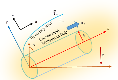
A two-dimensional, unsteady, MHD, laminar Casson and Williamson fluids with nano-particle over an inclined cylindrical surface is taken. B0 is uniform external magnetic field, which is applied to the cylinder which is occupied to electrically non-conducting. However, the impact of radiation and chemical reaction are also assumed in the boundary layer flows. Here, x and r axes are chosen along upward and normal direction respectively (Figure 1).
Figure 1. Physical configuration
Here, $u_{0}$ is the uniform velocity. The surface temperature and concentration of cylinder are $\overline{\mathrm{T}}_{\mathrm{w}}$ and $\overline{\mathrm{C}}_{\mathrm{w}},$ where $\overline{\mathrm{T}}_{\mathrm{w}}>\overline{\mathrm{T}}_{\infty}$ and $\bar{C}_{w}>\bar{C}_{\infty} .$ Under these assumptions, the decent model for Casson and Williamson nanofluid past an inclined cylindrical surface is taken in the form as,
Continuity Equation,
$\frac{\partial(\mathrm{ru})}{\partial \mathrm{x}}+\frac{\partial(\mathrm{rv})}{\partial \mathrm{r}}=0$ (1)
Momentum Equation,
$\frac{\partial u}{\partial \bar{t}}+u \frac{\partial u}{\partial x}+v \frac{\partial u}{\partial r}=q \upsilon\left(1+\frac{1}{\beta}\right)\left(\frac{\partial^{2} u}{\partial r^{2}}+\frac{1}{r} \frac{\partial u}{\partial r}\right)+(1-q) \upsilon$
$\left\{\frac{\partial^{2} u}{\partial r^{2}}+\frac{1}{r} \frac{\partial u}{\partial r}+\sqrt{2} \Gamma \frac{\partial u}{\partial r} \frac{\partial^{2} u}{\partial r^{2}}+\frac{\Gamma}{\sqrt{2} r}\left(\frac{\partial u}{\partial r}\right)^{2}\right\}$
$+g \beta_{T}\left(\bar{T}-\bar{T}_{\infty}\right) \operatorname{Cos} \alpha+g \beta_{C}\left(\bar{C}-\bar{C}_{\infty}\right) \cos \alpha-\frac{\sigma B_{0}^{2}}{\rho} u$ (2)
Energy Equation,
$\frac{\partial \overline{\mathrm{T}}}{\partial \overline{\mathrm{t}}}+\mathrm{u} \frac{\partial \overline{\mathrm{T}}}{\partial \mathrm{x}}+\mathrm{v} \frac{\partial \overline{\mathrm{T}}}{\partial \mathrm{r}}=\frac{\kappa}{\rho \mathrm{c}_{\mathrm{p}}}\left(\frac{\partial^{2} \overline{\mathrm{T}}}{\partial \mathrm{r}^{2}}+\frac{1}{\mathrm{r}} \frac{\partial \overline{\mathrm{T}}}{\partial \mathrm{r}}\right)+\frac{\sigma \mathrm{B}_{0}^{2} \mathrm{u}^{2}}{\rho \mathrm{c}_{\mathrm{p}}}$
$+\tau\left[\mathrm{D}_{\mathrm{B}} \frac{\partial \overline{\mathrm{C}}}{\partial \mathrm{r}} \frac{\partial \overline{\mathrm{T}}}{\partial \mathrm{r}}+\left(\frac{\mathrm{D}_{\mathrm{T}}}{\overline{\mathrm{T}_{\infty}}}\right)\left(\frac{\partial \overline{\mathrm{T}}}{\partial \mathrm{r}}\right)^{2}\right]-\frac{1}{\rho \mathrm{c}_{\mathrm{p}}} \frac{1}{\mathrm{r}} \frac{\partial}{\partial \mathrm{r}}(\mathrm{rq_r})$ (3)
Concentration Equation,
$\frac{\partial \overline{\mathrm{C}}}{\partial \overline{\mathrm{t}}}+\mathrm{u} \frac{\partial \overline{\mathrm{C}}}{\partial \mathrm{x}}+\mathrm{v} \frac{\partial \overline{\mathrm{C}}}{\partial \mathrm{r}}=\mathrm{D}_{\mathrm{B}}\left(\frac{\partial^{2} \overline{\mathrm{C}}}{\partial \mathrm{r}^{2}}+\frac{1}{\mathrm{r}} \frac{\partial \overline{\mathrm{C}}}{\partial \mathrm{r}}\right)$
$+\left(\frac{\mathrm{D}_{\mathrm{T}}}{\overline{\mathrm{T}_{\infty}}}\right)\left(\frac{\partial^{2} \overline{\mathrm{T}}}{\partial \mathrm{r}^{2}}+\frac{1}{\mathrm{r}} \frac{\partial \overline{\mathrm{T}}}{\partial \mathrm{r}}\right)-\overline{\mathrm{K}}\left(\overline{\mathrm{C}}-\overline{\mathrm{C}}_{\infty}\right)$ (4)
with,
$\overline{\mathrm{t}} \leq 0: \mathrm{u}=\mathrm{v}=0, \overline{\mathrm{T}}=\overline{\mathrm{T}}_{\infty,} \overline{\mathrm{C}}=\overline{\mathrm{C}}_{\infty}$
for all $\mathrm{x} \geq 0$ and $\mathrm{r} \geq 0$
$\overline{\mathrm{t}}>0: \mathrm{u}=\mathrm{u}_{0}, \mathrm{v}=0$
$-\kappa \frac{\partial \overline{\mathrm{T}}}{\partial \mathrm{r}}=\mathrm{h}_{\mathrm{f}}\left(\overline{\mathrm{T}}_{\mathrm{w}}-\overline{\mathrm{T}}_{\infty}\right), \overline{\mathrm{C}}=\overline{\mathrm{C}}_{\mathrm{w}}$ at $\mathrm{r}=\mathrm{r}_{0}$
$\mathrm{u}=\mathrm{v}=0, \overline{\mathrm{T}}=\overline{\mathrm{T}}_{\infty,} \overline{\mathrm{C}}=\overline{\mathrm{C}}_{\infty} \quad$ at $\mathrm{x}=0$
and $\mathrm{r} \geq \mathrm{r}_{0}$
$\mathbf{u} \rightarrow 0, \overline{\mathbf{T}} \rightarrow \overline{\mathrm{T}}_{\infty}, \overline{\mathbf{C}} \rightarrow \overline{\mathrm{C}}_{\infty} \quad$ as $\mathbf{r} \rightarrow \infty$ (5)
Here, a non-dimensional parameter $\mathrm{q} \in[0,1]$ is proposed to bend the momentum equation to Casson fluid flow when $q=$ 1 and Williamson fluid flow when $\mathrm{q}=0, \alpha$ is the inclination of the cylinder about x-axis, Casson fluid parameter is denoted by $\beta, \Gamma$ is rate time constant and $\upsilon \quad q_{\mathrm{r}}=\left(-4 \sigma_{\mathrm{s}} \overline{\mathrm{T}}^{4} / 3 \kappa_{\mathrm{e}} \partial r\right)$ is the radiative heat flux obtained by imposing Roseland approximation. Assuming small temperature differences inside the flow and expanding $\overline{\mathrm{T}}^{4}$ in Taylor series at $\overline{\mathrm{T}}_{\infty},$ we adopt, $\overline{\mathrm{T}}^{4} \cong 4 \overline{\mathrm{T}}_{\infty}^{3} \overline{\mathrm{T}}-3 \overline{\mathrm{T}}_{\infty}^{4}$ ( higher terms are omitted).
In view of Eq. (3) reduce to
$\frac{\partial \overline{\mathrm{T}}}{\partial \overline{\mathrm{t}}}+\mathrm{u} \frac{\partial \overline{\mathrm{T}}}{\partial \mathrm{x}}+\mathrm{v} \frac{\partial \overline{\mathrm{T}}}{\partial \mathrm{r}}=\frac{\kappa}{\rho \mathrm{c}_{\mathrm{p}}}\left(\frac{\partial^{2} \overline{\mathrm{T}}}{\partial \mathrm{r}^{2}}+\frac{1}{\mathrm{r}} \frac{\partial \overline{\mathrm{T}}}{\partial \mathrm{r}}\right)+\frac{\sigma \mathrm{B}_{0}^{2} \mathrm{u}^{2}}{\rho \mathrm{c}_{\mathrm{p}}}$
$+\tau\left[D_{B} \frac{\partial \bar{C}}{\partial r} \frac{\partial \bar{T}}{\partial r}+\left(\frac{D_{T}}{\overline{{T}_{\infty}}}\right)\left(\frac{\partial \bar{T}}{\partial r}\right)^{2}\right]+\frac{16 \sigma_{s} \bar{T}_{\infty}^{3}}{3 \kappa_{e} \rho c_{p}} \frac{1}{r} \frac{\partial}{\partial r}\left(r \frac{\partial \bar{T}}{\partial r}\right)$ (6)
Now the dimensionless elements are introduced as:
$\begin{aligned} \mathrm{X}=\frac{\mathrm{x \upsilon}}{\mathrm{u}_{0} \mathrm{r}_{0}^{2}}, & \mathrm{R}=\frac{\mathrm{r}}{\mathrm{r}_{0}}, \mathrm{U}=\frac{\mathrm{u}}{\mathrm{u}_{0}}, \mathrm{V}=\frac{\mathrm{vr}_{0}}{\mathrm{\upsilon}}, \mathrm{t}=\frac{\mathrm{\bar{t} \upsilon}}{\mathrm{r}_{0}^{2}} \\ \mathrm{T}=& \frac{\overline{\mathrm{T}}-\overline{\mathrm{T}}_{\infty}}{\overline{\mathrm{T}}_{\mathrm{w}}-\overline{\mathrm{T}}_{\infty}}, \mathrm{C}=\frac{\overline{\mathrm{C}}-\overline{\mathrm{C}}_{\infty}}{\overline{\mathrm{C}}_{\mathrm{w}}-\overline{\mathrm{C}}_{\infty}} \end{aligned}$
Using Eq. (6) and the above non-dimensional quantities, Eqns. (1)-(4) reduce into the dimensionless form,
Continuity Equation,
$\frac{\partial(\mathrm{RU})}{\partial \mathrm{X}}+\frac{\partial(\mathrm{RV})}{\partial \mathrm{R}}=0$ (7)
Momentum Equation,
$\frac{\partial \mathrm{U}}{\partial \mathrm{t}}+\mathrm{U} \frac{\partial \mathrm{U}}{\partial \mathrm{X}}+\mathrm{V} \frac{\partial \mathrm{U}}{\partial \mathrm{R}}=\mathrm{q}\left(1+\frac{1}{\beta}\right)\left(\frac{\partial^{2} \mathrm{U}}{\partial \mathrm{R}^{2}}+\frac{1}{\mathrm{R}} \frac{\partial \mathrm{U}}{\partial \mathrm{R}}\right)$
$+(1-q)\left\{\frac{\partial^{2} U}{\partial R^{2}}+\frac{1}{R} \frac{\partial U}{\partial R}+2 \lambda \frac{\partial U}{\partial R} \frac{\partial^{2} U}{\partial R^{2}}+\lambda \frac{1}{R}\left(\frac{\partial U}{\partial R}\right)^{2}\right\}$
$+\mathrm{GrTCos} \alpha+\mathrm{GmCCos} \alpha-\mathrm{MU}$ (8)
Energy Equation,
$\frac{\partial \mathrm{T}}{\partial \mathrm{t}}+\mathrm{U} \frac{\partial \mathrm{T}}{\partial \mathrm{X}}+\mathrm{V} \frac{\partial \mathrm{T}}{\partial \mathrm{R}}=\frac{1}{\operatorname{Pr}}\left(1+\frac{4}{3 \mathrm{R}}\right)\left(\frac{\partial^{2} \mathrm{T}}{\partial \mathrm{R}^{2}}+\frac{1}{\mathrm{R}} \frac{\partial \mathrm{T}}{\partial \mathrm{R}}\right)$
$+\mathrm{Nb}\left(\frac{\partial \mathrm{T}}{\partial \mathrm{R}}\right)\left(\frac{\partial \mathrm{C}}{\partial \mathrm{R}}\right)+\mathrm{Nt}\left(\frac{\partial \mathrm{T}}{\partial \mathrm{R}}\right)^{2}+\mathrm{EcMU}^{2}$ (9)
Concentration Equation,
$\frac{\partial \mathrm{C}}{\partial \mathrm{t}}+\mathrm{U} \frac{\partial \mathrm{C}}{\partial \mathrm{X}}+\mathrm{V} \frac{\partial \mathrm{C}}{\partial \mathrm{R}}=\frac{1}{\mathrm{Le}}\left\{\left(\frac{\partial^{2} \mathrm{C}}{\partial \mathrm{R}^{2}}+\frac{1}{\mathrm{R}} \frac{\partial \mathrm{C}}{\partial \mathrm{R}}\right)\right.$$\left.+\left(\frac{\mathrm{Nt}}{\mathrm{Nb}}\right)\left(\frac{\partial^{2} \mathrm{T}}{\partial \mathrm{R}^{2}}+\frac{1}{\mathrm{R}} \frac{\partial \mathrm{T}}{\partial \mathrm{R}}\right)\right\}-\mathrm{KC}$ (10)
And the corresponding boundary criterions in terms of dimensionless variables are,
$\mathrm{t} \leq 0: \mathrm{U}=0, \mathrm{V}=0, \mathrm{T}=0, \mathrm{C}=0 \quad$ everywhere
$\mathrm{t}>0: \mathrm{U}=1, \mathrm{V}=0, \frac{\partial \mathrm{T}}{\partial \mathrm{R}}=-\gamma, \mathrm{C}=1 \quad$ at $\mathrm{R}=1$
$\begin{array}{l}{\mathrm{U}=0, \mathrm{V}=0, \mathrm{T}=0, \mathrm{C}=0 \quad \text { at } \mathrm{X}=0 \text { and } \mathrm{R} \geq 1} \\{\mathrm{U} \rightarrow 0, \mathrm{V} \rightarrow 0, \mathrm{T} \rightarrow 0, \mathrm{C} \rightarrow 0 \mathrm{at} \mathrm{R} \rightarrow \infty}\end{array}$ (11)
where, Williamson parameter, $\quad \lambda=\frac{\Gamma}{\sqrt{2}}\left(\frac{\mathrm{u}_{0}}{\mathrm{r}_{0}}\right) $, Magnetic parameter, $\quad \mathrm{M}=\frac{\sigma \mathrm{B}_{0}^{2} \mathrm{r}_{0}^{2}}{\rho \mathrm{\upsilon}} $ Thermal $\quad$ Grashof $\quad$ number $\mathrm{Gr}=\frac{\mathrm{g} \beta_{\mathrm{T}} \mathrm{r}_{0}^{2}\left(\overline{\mathrm{T}}_{\mathrm{w}}-\overline{\mathrm{T}}_{\infty}\right)}{\mathrm{u}_{0} \mathrm{\upsilon}},$ Biot number $\gamma=\frac{\mathrm{h}_{\mathrm{f}} \mathrm{r}_{0}}{\mathrm{\kappa}}, \quad$ Prandtl number, $\operatorname{Pr}=\frac{\rho \mathrm{c}_{\mathrm{p}} \mathrm{ \upsilon }}{\mathrm{\kappa}},$ Eckert number, $\mathrm{Ec}=\frac{\mathrm{u}_{0}^{2}}{\mathrm{c}_{\mathrm{p}}\left(\overline{\mathrm{T}}_{\mathrm{w}}-\overline{\mathrm{T}}_{\infty}\right)}$, radiation parameter, $\quad \mathrm{Ra}=\frac{\kappa_{\mathrm{e}} \kappa}{4 \sigma_{\mathrm{s}} \overline{\mathrm{T}}_{\infty}^{3}}, \quad$ Chemical reaction $\mathrm{K}=\frac{\overline{\mathrm{K}} \mathrm{r}_{0}^{2}}{\mathrm{\upsilon}},$ Brownian parameter, $\quad \mathrm{Nb}=\frac{\tau \mathrm{D}_{\mathrm{B}}\left(\overline{\mathrm{C}}_{\mathrm{w}}-\overline{\mathrm{C}}_{\mathrm{o}}\right)}{\mathrm{\upsilon}}$ thermophoresis parameter, $\quad \mathrm{Nt}=\frac{\tau \mathrm{D}_{\mathrm{T}}\left(\overline{\mathrm{T}}_{\mathrm{w}}-\overline{\mathrm{T}}_{\infty}\right)}{\overline{\mathrm{T}}_{\infty}\mathrm{v}}, \quad$ Lewis number, $\quad \mathrm{Le}=\frac{\upsilon}{\mathrm{D}_{\mathrm{B}}} \quad$ and $\quad$ mass $\quad$ Grashof $\quad$ number, $G r=\frac{g \beta_{C} r_{0}^{2}\left(\bar{C}_{w}-\bar{C}_{\infty}\right)}{u_{0} \upsilon}$
The physical non-dimensional quantities namely skin frictions, Nusselt and Sherwood numbers are chosen respectively by the following expressions
$C_{f}=-\frac{1}{2 \sqrt{2}} G r^{-3 / 4}\left(\frac{\partial U}{\partial R}\right)_{R=0}$ (12)
$\mathrm{Nu}=\frac{1}{\sqrt{2}} \mathrm{Gr}^{-3 / 4}\left(\frac{\partial \mathrm{T}}{\partial \mathrm{R}}\right)_{\mathrm{R}=0}$ (13)
$\mathrm{Sh}=\frac{1}{\sqrt{2}} \mathrm{Gr}^{-3 / 4}\left(\frac{\partial \mathrm{C}}{\partial \mathrm{R}}\right)_{\mathrm{R}=0}$ (14)
Stream function $\psi$ satisfied Eq. ( 1) and associated as, $\mathrm{U}=\frac{\partial \psi}{\partial \mathrm{Y}}, \mathrm{V}=-\frac{\partial \psi}{\partial \mathrm{X}}$.
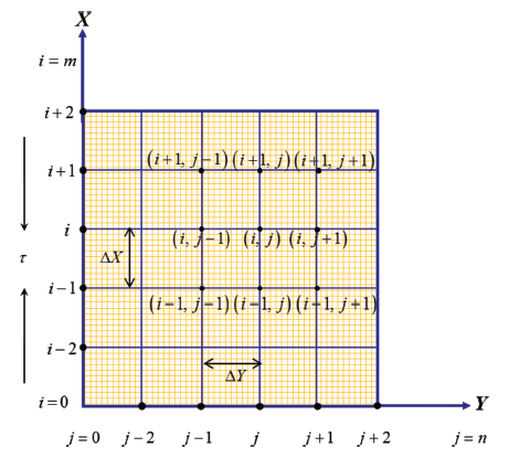
An explicit scheme [20-23] has been exerted to solve the Eqns. (7)-(11). A rectangular shape of flow region is being chosen for dividing the grid lines (Figure 2). For the remaining investigations, it is chosen as,
Grid space: M = 100, N = 200, Height of plates: Xmax = 20, Rmax = 50 as R→∞,
Mesh Size: $\Delta \mathrm{R}=0.251(0 \leq \mathrm{R} \leq 50)$ and $\Delta \mathrm{X}=0.202(0 \leq \mathrm{X} \leq 20)$, Δτ = 0.001.
Thus Eqns. (7)-(11) are transformed into the following form,
$\frac{\mathrm{U}(\mathrm{i}, \mathrm{j})-\mathrm{U}(\mathrm{i}-1, \mathrm{j})}{\Delta \mathrm{X}}+\frac{\mathrm{V}(\mathrm{i}, \mathrm{j})-\mathrm{V}(\mathrm{i}-1, \mathrm{j})}{\Delta \mathrm{R}}$ $+\frac{V(i, j)}{1+(j-1) \Delta R}=0$ (15)
$\frac{\mathrm{U}^{\prime}(\mathrm{i}, \mathrm{j})-\mathrm{U}(\mathrm{i}, \mathrm{j})}{\Delta \mathrm{t}}+\mathrm{U}(\mathrm{i}, \mathrm{j}) \frac{\mathrm{U}(\mathrm{i}, \mathrm{j})-\mathrm{U}(\mathrm{i}-1, \mathrm{j})}{\Delta \mathrm{X}}$
$+\mathrm{V}(\mathrm{i}, \mathrm{j}) \frac{\mathrm{U}(\mathrm{i}, \mathrm{j}+1)-\mathrm{U}(\mathrm{i}, \mathrm{j})}{\Delta \mathrm{R}}=+\operatorname{Gr} \mathrm{T}(\mathrm{i}, \mathrm{j}) \cos \alpha$
$\mathrm{q}\left(1+\frac{1}{\beta}\right)\left\{\frac{\mathrm{U}(\mathrm{i}, \mathrm{j}+1)-2 \mathrm{U}(\mathrm{i}, \mathrm{j})+\mathrm{U}(\mathrm{i}, \mathrm{j}-1)}{(\Delta \mathrm{R})^{2}}\right.$
$\left.+\frac{1}{1+(j-1) \Delta R} \frac{U(i, j+1)-U(i, j)}{\Delta R}\right\}+(1-q)$ $\left\{\frac{\mathrm{U}(\mathrm{i}, \mathrm{j}+1)-2 \mathrm{U}(\mathrm{i}, \mathrm{j})+\mathrm{U}(\mathrm{i}, \mathrm{j}-1)}{(\Delta \mathrm{R})^{2}}+\frac{1}{1+(\mathrm{j}-1) \Delta \mathrm{R}}\right.$
$\frac{\mathrm{U}(\mathrm{i}, \mathrm{j}+1)-\mathrm{U}(\mathrm{i}, \mathrm{j})}{\Delta \mathrm{R}}+2 \lambda \frac{\mathrm{U}(\mathrm{i}, \mathrm{j}+1)-\mathrm{U}(\mathrm{i}, \mathrm{j})}{\Delta \mathrm{R}}$
$+\frac{\lambda}{\mathrm{R}}\left(\frac{\mathrm{U}(\mathrm{i}, \mathrm{j}+1)-\mathrm{U}(\mathrm{i}, \mathrm{j})}{\Delta \mathrm{R}}\right)^{2}-\mathrm{MU}(\mathrm{i}. \mathrm{j})+\mathrm{GmC}(\mathrm{i}, \mathrm{j}) \cos \alpha$ (16)
$\frac{\mathrm{T}^{\prime}(\mathrm{i}, \mathrm{j})-\mathrm{T}(\mathrm{i}, \mathrm{j})}{\Delta \mathrm{t}}+\mathrm{U}(\mathrm{i}, \mathrm{j}) \frac{\mathrm{T}(\mathrm{i}, \mathrm{j})-\mathrm{T}(\mathrm{i}-1, \mathrm{j})}{\Delta \mathrm{X}}$
$+V(i, j) \frac{T(1, j+1)-T(i, j)}{\Delta R}=\frac{1}{\operatorname{Pr}}\left(1+\frac{4}{3 R a}\right)$
$\left\{\frac{\mathrm{T}(\mathrm{i}. \mathrm{j}+1)-2 \mathrm{T}(\mathrm{i}, \mathrm{j})+\mathrm{T}(\mathrm{i}, \mathrm{j}-1)}{(\Delta \mathrm{R})^{2}}+\frac{1}{1+(\mathrm{j}-1) \Delta \mathrm{R}}\right.$
$\left.\frac{\mathrm{T}(\mathrm{i}, \mathrm{j}+1)-\mathrm{T}(\mathrm{i}, \mathrm{j})}{\Delta \mathrm{R}}\right\}+\mathrm{Nb}\left\{\frac{\mathrm{T}(\mathrm{i}, \mathrm{j}+1)-\mathrm{T}(\mathrm{i}, \mathrm{j})}{\Delta \mathrm{R}}\right\}$
$\left\{\frac{\mathrm{C}(\mathrm{i}, \mathrm{j}+1)-\mathrm{C}(\mathrm{i}, \mathrm{j})}{\Delta \mathrm{R}}\right\}+\mathrm{Nt}\left\{\frac{\mathrm{T}(\mathrm{i}, \mathrm{j}+1)-\mathrm{T}(\mathrm{i}, \mathrm{j})}{\Delta \mathrm{R}}\right\}^{2}+\mathrm{EcM}(\mathrm{U}(\mathrm{i}, \mathrm{j}))^{2}$ (17)
$\frac{\mathrm{C}(\mathrm{i}, \mathrm{j})-\mathrm{C}(\mathrm{i}, \mathrm{j})}{\Delta \mathrm{t}}+\mathrm{U}(\mathrm{i}, \mathrm{j}) \frac{\mathrm{C}(\mathrm{i}, \mathrm{j})-\mathrm{C}(\mathrm{i}-1, \mathrm{j})}{\Delta \mathrm{X}}$
$+V(i, j) \frac{C(i, j+1)-C(i, j)}{\Delta R}=\frac{1}{L e}\left\{\frac{C(i. j+1)-2 C(i, j)+C(i, j-1)}{(\Delta R)^{2}}\right.$
$\left.+\frac{1}{1+(j-1) \Delta R} \frac{C(i, j+1)-C(i, j)}{\Delta R}\right\}+\left(\frac{N t}{N b}\right)$
$\left\{\frac{\mathrm{T}(\mathrm{i}. \mathrm{i}+1)-2 \mathrm{T}(\mathrm{i}, \mathrm{j})+\mathrm{T}(\mathrm{i}, \mathrm{j}-1)}{(\Delta \mathrm{R})^{2}}+\frac{1}{1+(\mathrm{j}-1) \Delta \mathrm{R}} \frac{\mathrm{T}(\mathrm{i}, \mathrm{j}+1)-\Delta(\mathrm{i}, \mathrm{j})}{\Delta \mathrm{R}}\right\}$
$-\mathrm{KC}(\mathrm{i}, \mathrm{j})$ (18)
$\mathrm{U} \frac{\Delta \mathrm{t}}{\Delta \mathrm{X}}+\mathrm{V} \frac{\Delta \mathrm{t}}{\Delta \mathrm{R}}+\frac{1}{\operatorname{Pr}}\left(1+\frac{4}{3 \mathrm{Ra}}\right)\left\{\frac{2 \Delta \mathrm{t}}{(\Delta \mathrm{R})^{2}}+\frac{\Delta \mathrm{t}}{\mathrm{R} \Delta \mathrm{R}}\right\}$
$-\mathrm{CNb} \frac{2 \Delta \mathrm{t}}{(\Delta \mathrm{R})^{2}}-\mathrm{TNt} \frac{2 \Delta \mathrm{t}}{(\Delta \mathrm{R})^{2}} \leq 1$ (19)
and
$\mathrm{U} \frac{\Delta \mathrm{t}}{\Delta \mathrm{X}}+\mathrm{V} \frac{\Delta \mathrm{t}}{\Delta \mathrm{R}}+\frac{1}{\mathrm{Le}}\left\{\frac{2 \Delta \mathrm{t}}{(\Delta \mathrm{R})^{2}}+\frac{\Delta \mathrm{t}}{\mathrm{R} \Delta \mathrm{R}}\right\}+\frac{\mathrm{K}}{2} \Delta \mathrm{t} \leq 1$ (20)
with,
when, $\mathrm{t} \leq 0$ then, $\mathrm{U}_{\mathrm{j}}^{0}=0, \mathrm{T}_{\mathrm{j}}^{0}=0, \mathrm{C}_{\mathrm{j}}^{0}=0,$ everywhere
when, $\mathrm{t}>0$ then, $\mathrm{U}_{\mathrm{j}}^{0}=1, \mathrm{T}_{\mathrm{j}}^{0}=\gamma \Delta \mathrm{R}+\mathrm{T}_{\mathrm{j}+1}^{0}, \mathrm{C}_{\mathrm{j}}^{0}=1,$ for all $\mathrm{R}=1$
$\mathrm{U}_{\mathrm{j}}^{\mathrm{n}}=0, \mathrm{T}_{\mathrm{j}}^{\mathrm{n}}=0, \mathrm{C}_{\mathrm{j}}^{\mathrm{n}}=0 \text { as } \mathrm{R} \rightarrow \infty$
The stability criterions can be achieved after simplification as, [24-28]
Figure 2. Finite difference space
Using the initial condition U=V=T=C=0 at τ= 0 and for, ΔX= 0.202, ΔR= 0.251 and Δτ= 0.001, the stability postulate for the ongoing research would be formed as, Pr≥0.52 and Le≥0.036.
Unsteady hydromagnetic 2D Casson and Williamson fluids flow over an inclined cylinder has been investigated numerically. The physical significance of diversified flow fields has been exhibited for different pertinent parameters. The value of the main parameters is considered as M=1.0, Pr=0.71 (for air), $\gamma=0.2, \beta=\lambda=0.1$, Nt=Nb=0.1, Gm=Gr =5.0, $\alpha=\pi / 3$, K=0.5, Ra=0.1, Ec=0.001 and Le=1.0. However, the advanced visualisations of fluid flows are also depicted through isotherms and streamlines. However, the numerical validation of this work is self-evident in Table 1 and 2 respectively.
Table 1. Comparison of Nu for various parameter of Pr, Gr=Gm=M=Le=Nb=Nt=K=Ec=α=Ra=0.when q=1 (Casson fluid)
|
Pr |
Present results |
Previous results [19] |
|
0.2 |
0.16897 |
0.1691 |
|
0.7 |
0.45304 |
0.4538 |
|
2.0 |
0.91807 |
0.9113 |
Table 2. Comparison of Nu for various parameter of Pr, when q=0 (Williamson fluid) λ=Gr=Gm=M=Le=Nb=Nt=K=Ec=α=Ra=0
|
Pr |
Present results |
Previous results [12] |
|
0.2 |
0.16897 |
0.169522 |
|
0.7 |
0.45304 |
0.453916 |
|
2.0 |
0.91807 |
0.911358 |
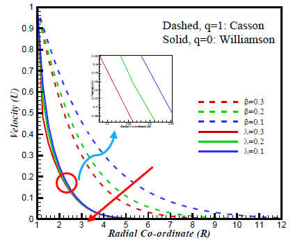
Physically, Casson fluid parameter, $\beta$, has a tendency to increase fluid viscosity. Similarly, increment of Williamson fluid parameter, $\lambda$, the time relaxation of fluid develops that leads an obstacle to fluid particle and therefore velocity profiles decrease. Figure 3 shows that the momentum boundary layers of Williamson fluid decrease more than that of the Casson fluid since the flow resistance is comparatively greater on Williamson fluid.
Figure 3. Impact of λ and β on U
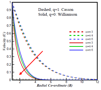
Figure 4. Impact of $\alpha$ on U
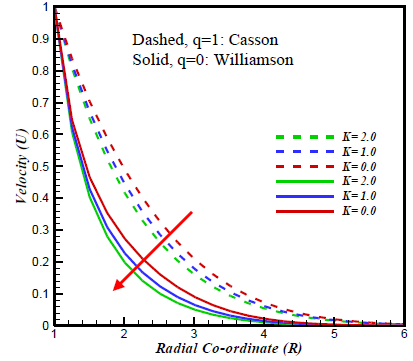
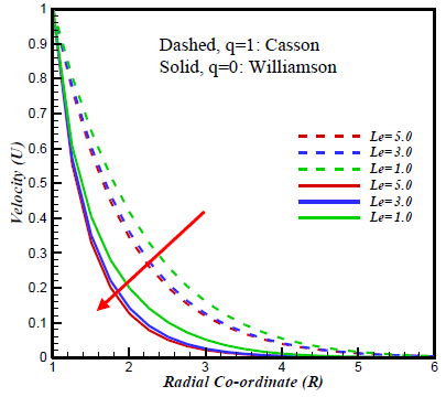
If the inclination about x-axis increases, the effects of gravity decreases, due to this velocity fields decline with in the boundary layer (Figure 4). The effect of velocity profile has been shown for diversified data of magnetic parameter, M (Figure 5). It is examined that the field of velocity diminishes for increasing M. This is because, high intensity of magnetic term assists to develop a declining force (Lorentz force), which diminish the fluid motion. The red line exhibits no impression of M. It is clear that Lorentz force influenced Williamson fluid effectively rather than Casson fluid. Figure 6 indicates the impression of chemical reaction, K on velocity fields and it is seen that for the presence of K, Williamson fluid velocity is more reducing compared with the Casson fluid velocity at R=3. The curve to curve decreasing rate for Casson fluid is 3.0% from K=0.0 to 1.0, 1.8% from K =1.0 to 2.0 and for Williamson fluid 3% from K=0.0 to 1.0 and 1.0% from K =1.0 to 2.0. Lewis number Le is directly proportional to the kinematic viscosity, $\upsilon$, and when $\upsilon$ improves velocity profiles decrease for both fluid phases. It is observed that increasing values of Le momentum boundary layers for Williamson fluid decrease more compared to that of Casson fluid (Figure 7).
Figure 5. Impact of M on U
Figure 6. Impact of K on U
Figure 7. Impact of Le on U
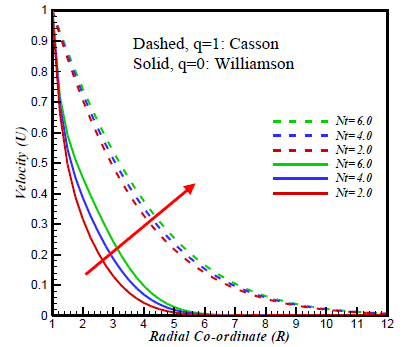
On the other hand, thermophoresis parameter, Nt, is inversely proportional to the kinematic viscosity υ. Therefore, the developing values of Nt, velocity profiles improve and momentum boundary layers for Williamson fluid decrease more than that of Casson fluid, depicted in Figure 8.
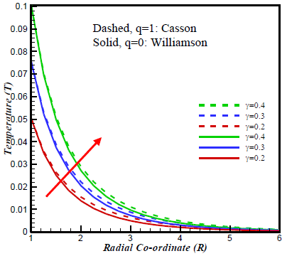
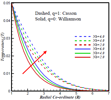
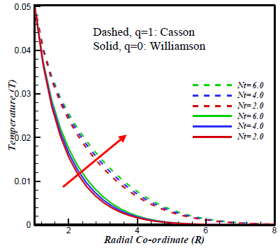
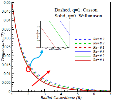
Figure 9, is displayed to represent the variation of boundary layers on temperature field for the impact of Biot number, γ. An increment of, γ, coefficient of heat transfer, hs, enrich and the more hs increase, the heat is more transferred from hotter surface to the cooler surface of the cylinder and corresponding boundary layer thickness aggravate. Figures 10-11 represent the temperature profiles for diversified values of Brownian, Nb, and thermophoresis, Nt, parameters respectively. Physically, developing Nb and Nt have the tendency to accelerate fluid particles motion and eventually develops the fluid temperature. Here, Casson fluid got influenced significantly for both parameters than Williamson fluid. The behaviour of the temperature fields for distinct data of Radiation parameter, Ra, is demonstrated in Figure 12. It is examined that, Ra is directly proportional to thermal conductivity, $\kappa$. Thus, due to the increment of Ra, thermal boundary layers increase at high level for Casson fluid compared to Williamson fluid. Due to the storage of energy at high Eckert number, Ec, the particles become operative and lead to higher temperature, and Casson fluid behaves more actively than the other one (Figure 13).
Figure 8. Impact of Nt on U
Figure 9. Impact of $\gamma$ on T
Figure 10. Impact of Nb on T
Figure 11. Impact of Nt on T
Figure 12. Impact of Ra on T
The impression of Nt, on concentric fields, are exhibited in Figure 14. Also, it is exhibited that the concentric boundary layers for Williamson fluid increase more than that of Casson fluid. The effect of skin friction has been displayed in Figures 15-16 for distinct data of β, $\lambda$ and M respectively. For the increase of the parameter β, $\lambda$ and M, skin friction declines. For the development in β and $\lambda$, viscosity of the fluid rises. Therefore, skin friction decreases
Figure 13. Impact of Ec on T
Figure 14. Impact of Nt on C
Figure 15. Impact of $\lambda$ and $\beta$ on skin friction profiles
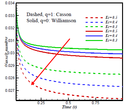
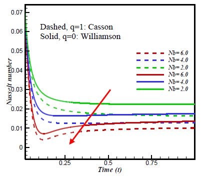
Figures 17-19 identify that, there is an inverse relation among the Nusselt number to the respective parameters on the mentioned graph. Moreover, it is observed that Nusselt number got influence more effectively by Williamson fluid compared to Casson fluid.
Figure 16. Impact of M on skin friction profiles
Figure 17. Impact of Ec on Nusselt number profiles
Figure 18. Impact of Nb on Nusselt number profiles
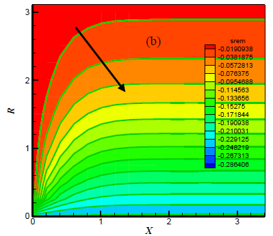
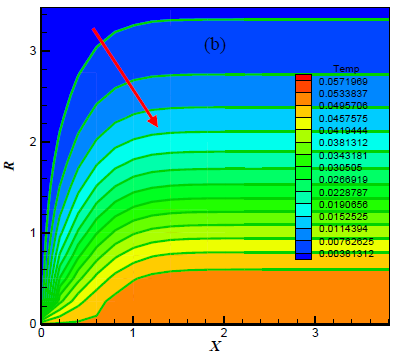
The updated visualisation of fluid fields can be exhibited with the help of streamlines. However, the changes of thermal boundary layer can be presented through isotherms. The impressions of streamlines as well as isotherms are illustrated in Figures 20-21. Streamlines and isotherms both decrease with the increase of both parameter from β = $\lambda$=0.1 to 0.2. Figure 20(a) and Figure 21(a) are representing the line view, on the other hand, Figure 20(b) and Figure 21(b) are the contour flood view.
Figure 19. Impact of Nt on Nusselt number profiles
Figure 20. (a) Streamlines for Casson fluid when $\beta=0.2$ (red dashed line) and $\beta=0.1$ (green solid line) and (b) Streamlines flood view for Williamson fluid when $\lambda=0.2$ and $\lambda=0.1$
Figure 21. (a) Isotherms for Casson fluid when $\beta=0.2$ (red dashed line) and $\beta=0.1$ (solid green line) and (b) flood view for Williamson fluid when $\lambda=0.2$ and $\lambda=0.1$
A comparison between chemically reactive Casson and Williamson radiative nanofluids past an inclined cylindrical surface are investigated here. A validation of this study against previously published literature is also presented. The critical observations are concluded below:
B0 external magnetic field, $\left[\mathrm{Wbm}^{-2}\right]$
Cf skin friction, [-]
$\bar{C}$ concentration component
C dimensionless concentration [-]
$\bar{C}_{W}$ concentration of the cylinder, [mol.]
$\overline{\mathrm{C}}_{\infty}$ concentration away from the cylinder
DB coefficient of Brownian diffusion
DT coefficient of thermophoresis diffusion
Ec Eckert number, [-]
g Gravitational acceleration, $\left[\mathrm{ms}^{-2}\right]$
Gr thermal Grashof number, [-]
hf heat transfer coefficient, $\left[\mathrm{W} /\left(\mathrm{m}^{2} \mathrm{K}\right)\right]$
K chemical reaction, [-]
Le Lewis number, [-]
M magnetic parameter, [-]
Nu Nusselt number, [-]
Nt thermophoresis parameter, [-]
Nb Brownian parameter, [-]
Pr Prandlt number, [-]
qr radiative heat flux, [ $\mathrm{kgm}^{-2}$ ]
R radial direction
Ra radiation parameter, [-]
Sh Sherwood number, [-]
$\bar{T}$ temperature, [K]
T dimensionless temperature [-]
$\overline{\mathrm{T}}_{\mathrm{w}}$ temperature outside the boundary layer
$\bar{t}$ dimensional time, [s]
u,v dimensional velocity of the fluid in x and r direction
U dimensionless velocity [-]
Greek symbols
α inclined angle
β Casson parameter, [-]
γ Biot number, [-]
Γ rate time constant, [s]
κ thermal conductivity, [$\mathrm{Wm}^{-1} \mathrm{K}^{-1}$]
λ Williamson parameter, [-]
ρ density, [$\mathrm{kgm}^{-3}$]
σS Stefan-Boltzmann constant, [$\mathrm{Wm}^{2} \mathrm{K}^{-4}$]
υ kinematic viscosity, [ $m^{2} s^{-1}$]
[1] Casson, N. (1959). A flow equation for pigment oil suspensions of the printing ink type. Open Journal of Fluid Dynamics, 6(4): 84-102.
[2] Hussanan, A., Zukhi, S.M., Tahar, R.M., Khan, I. (2014). Unsteady boundary layer flow and heat and mass transfer of a Casson fluid past an oscillating vertical plate with Newtonian heating. PLOS ONE, 9: e108763. https://doi.org/10.1371/journal.pone.0108763
[3] Malik, M.Y., Naseer, M., Nadeem, S., Rehman, A. (2014). The boundary layer flow of Casson nanofluid over a vertical exponentially stretching cylinder. Applied Nanoscience, 4: 869-873. https://doi.org/10.1007/s13204-013-0267-0
[4] Hayat, T., Bilal, A.M., Shehzad, S.A., Alsaedi, A. (2015). Mixed convection flow of Casson nanofluid over a stretching sheet with convectively heated chemical reaction and heat source/sink. Journal of Applied Fluid Mechanics, 8: 803-811. https://doi.org/10.18869/acadpub.jafm.67.223.22995
[5] Makanda, G., Shaw, S., Sibanda, P. (2015). Effects of radiation on MHD free convection of a Casson fluid from a horizontal circular cylinder with partial slip in non-Darcy porous medium with viscous dissipation. Boundary Value Problems, 2015: 75. https://doi.org/10.1186/s13661-015-0333-5
[6] Kataria, H.R., Patal, H.R. (2016). Soret and heat generation effects on MHD Casson fluid flow past an oscillating vertical plate embedded through porous medium. Alexandria Engineering Journal, 55: 2125-2137. https://doi.org/10.1016/j.aej.2016.06.024
[7] Kataria, H.R., Patel, H.R. (2016). Radiation and chemical reaction effects on MHD Casson fluid flow past an oscillating vertical plate embedded in porous medium. Alexandria Engineering Journal, 55: 583-595. https://doi.org/10.1016/j.aej.2016.01.019
[8] Ahmed, A.A. (2017). The influence of slip boundary condition on Casson nanofluid flow over a stretching sheet in the presence of viscous dissipation and chemical reaction. Hindawi, 2017: 1-12. https://doi.org/10.1155/2017/3804751
[9] Bhattacharyya, K. (2013). MHD stagnation-point flow of Casson fluid and heat transfer over a stretching sheet with thermal radiation. Journal of Thermodynamics, 2013: 1-9. http://dx.doi.org/10.1155/2013/169674
[10] Tamoor, M., Waqas, M., Khan, M.I., Alsaedi, A., Hayat, T. (2017). Magnetohydrodynamic flow of Casson fluid over a stretching cylinder. Results in Physics, 7: 498-502. https://doi.org/10.1016/j.rinp.2017.01.005
[11] Williamson, R.V. (1929). The flow of pseudoplastic materials. Ind. Eng. Chen., 21: 1108-1111. https://doi.org/10.1021/ie50239a035
[12] Venkataramanaiah, G., Sreedharbabu, M., Lavanya, M. (2016). Heat generation/absorption effects of magneto Williamson nanofluids flow with heat and mass fluxes. International Journal of Engineering Development and Research, 4: 284-297. https://doi.org/10.5281/zenodo.1316239
[13] Khan, M.S., Rahman, M.M., Arifuzzaman, S.M., Biswas, P., Karim, I. (2017). Williamson fluid flow behaviour of MHD convective-radiative Cattaneo-Christov heat flux type over a linearly stretched-surface with heat generation and thermal-diffusion. Frontiers in Heat and Mass Transfer, 9: 1-11. https://doi.org/10.5098/hmt.9.15
[14] Kothandapani, M., Prakash, J. (2015). Effects of thermal radiation parameter and magnetic field and the peristaltic motion of Williamson nanofluids in a tapered asymmetric channel. International Journal of Heat and Mass Transfer, 81: 234-245. https://doi.org/10.1016/j.ijheatmasstransfer.2014.09.062
[15] Abegunrin, O.A., Okhuevbie, S.O., Animasaun, I.L. (2016). Comparison between the flow of two non-Newtonian fluids over an upper horizontal surface of paraboloid of revolution: Boundary layer analysis. Alexandria Engineering Journal, 55: 1915-1929. https://doi.org/10.1016/j.aej.2016.08.002
[16] Kumaran, G., Sandeep, N. (2016). Computational analysis of magnetohydrodynamic Casson and Maxwell flows over a stretching sheet with cross diffusion. Results in Physics, 7: 147-155. https://doi.org/10.1016/j.rinp.2016.12.011
[17] Kumaran, G., Sandeep, N. (2017). Thermophoresis and Brownian moment effects on parabolic flow of MHD Casson and Williamson fluids with cross diffusion. Journal of Molecular Liquids, 233: 262-269. https://doi.org/10.1016/j.molliq.2017.03.031
[18] Mondal, R.N., Islam, S., Uddin, K., Hossain, A. (2013). Effects of aspect ratio on unsteady solutions through curved duct flow. Applied Mathematics and Mechanics 34(9): 1107-1122. https://doi.org/10.1007/s10483-013-1731-8
[19] Afify, A.A. (2017). The influence of slip boundary condition on Casson nanofluid flow over a stretching sheet in the presence of viscous dissipation and chemical reaction. Mathematical Problems in Engineering, 2017: 12. https://doi.org/10.1155/2017/3804751
[20] Arifuzzaman, S.M., Khan, M.S., Mamun, A.A., Reza-E-Rabbi, S., Biswas, P.F., Karim, I. (2019). Hydrodynamic stability and heat and mass transfer flow analysis of MHD radiative fourth-grade fluid through porous plate with chemical reaction. J. King Saud Univ. Sci., 31(4): 1388-1398. https://doi.org/10.1016/j.jksus.2018.12.009
[21] Arifuzzaman, S.M., Khan, M.S., Mehedi, M.F.U., Rana, B.M.J., Ahmmed, S.F. (2018). Chemically reactive and naturally convective high speed MHD fluid flow through an oscillatory vertical porous plate with heat and radiation absorption effect. Engineering Science and Technology, an International Journal, 21: 215-228. https://doi.org/10.1016/j.jestch.2018.03.004
[22] Bég, O.A., Khan, M.S., Karim, I., Alam, M.M., Ferdows, M. (2014). Explicit numerical study of unsteady hydromagnetic mixed convective nanofluid flow from an exponentially stretching sheet in porous media. Applied Nanoscience, 4: 943-957. https://doi.org/10.1007/s13204-013-0275-0
[23] Reza-E-Rabbi, S., Arifuzzaman, S. M., Sarkar, T., Khan, M. S., Ahmmed, S.F. (2018). Explicit finite difference analysis of an unsteady MHD flow of a chemically reacting Casson fluid past a stretching sheet with Brownian motion and thermophoresis effects. J. King Saud Univ. Sci., Article in Press. https://doi.org/10.1016/j.jksus.2018.10.017
[24] Reza-E-Rabbi, S., Ahmmed, S.F., Arifuzzaman, S.M., Sarkar, T., Khan, M.S. (2019). Computational modeling of multiphase fluid flow behavior over a stretching sheet in presence of nanoparticles. Engineering Science and Technology, an International Journal in Press. https://doi.org/10.1016/j.jestch.2019.07.006
[25] Reza-E-Rabbi, S., Arifuzzaman, S.M., Sarkar, T., Khan, M.S., Ahmmed, S.F. (2019). Periodic magnetohydrodynamic simulation of Newtonian and non- Newtonian fluids flow behaviour past a stretching sheet with nanoparticles. AIP Conference Proceedings, 2121(1): 070006. https://doi.org/10.1063/1.5115913
[26] Mamun, A.A., Arifuzzaman, S.M., Reza-E-Rabbi, S., Biswas, P., Khan M.S. (2018). Numerical investigation of boundary-layer flow of Sisko nanofluids through a nonlinear stretching sheet with MHD and thermal radiation effects. International Journal of Heat and Technology, 37(1): 285-295. https://doi.org/10.18280/ijht.370134
[27] Sarkar, T., Arifuzzaman, S.M., Reza-E-Rabbi, S., Khan, M.S., Ahmed, R., Ahmmed, S.F. (2018). Unsteady magnetohydrodynamic Casson nanofluid flow through a moving cylinder with Brownian and thermophoresis effects. Annales de Chimie: Science Des Materiaux, 42(2): 181-207. https://doi.org/10.3166/ACSM.42.181-207
[28] Sarkar, T., Arifuzzaman, S.M., Reza-E-Rabbi, S., Khan, M.S., Ahmed, R., Ahmmed, S.F. (2019). Computational modelling of chemically reactive and radiative flow of Casson-Carreau nanofluids over an inclined cylindrical surface with bended Lorentz force presence in porous medium. AIP Conference Proceedings, p. 050006. https://doi.org/10.1063/1.5115893