Yan Wang | Zhongshui Man*
© 2019 IIETA. This article is published by IIETA and is licensed under the CC BY 4.0 license (http://creativecommons.org/licenses/by/4.0/).
OPEN ACCESS
The finite volume method (FVM) can adapt to complex boundaries, achieve conservation of integrals, and generate flexible integral grids. Compared with the finite difference method (FDM), the FVM is immune to numerical oscillations and numerical dispersions. This paper aims to simulate the coalbed methane (CBM)-water two-phase flow in complex coal rock, and predict the CBM and water outputs in an accurate manner. Therefore, the FVM was introduced to create a simulation model of coalbed methane (CBM) productivity in 3D dual-porosity coal reservoir under non-equilibrium adsorption and pseudo-steady state conditions. The established model was applied to an actual project in Qinshui Basin, Shanxi Province, China. The historical gas and water outputs of a single CBM well were fitted with our model, and the simulated curves agree with the overall trend of the historical drainage and production curves. Next, the change trends of gas and water outputs in the CBM well were predicted, and the sensitivities of gas well productivity to three main reservoir parameters were analyzed. The results correctly reflect the productivity trend of the CBM well, indicating the correctness and feasibility of our model. Our research effectively simulates the migration of the CBM in coal rock with complex boundaries, providing a valuable reference for the development of the CBM.
coalbed methane (CBM) productivity, finite volume method (FVM), numerical simulation, influencing factors
The industrial and social development has brought a growing demand for energy. However, the conventional energy sources like oil and gas are dwindling. As a result, coalbed methane (CBM), an unconventional energy source, now plays an increasingly important role in energy consumption. Numerical simulation and prediction of coalbed methane production capacity are of great significance in block selection, economic evaluation, and production management [1]. Currently, the numerical simulations of the CBM are generally based on triple-porosity dual-permeability models that cover multiple components across the gas field. The partial differential equations or equation sets are often adopted as governing equations of the CBM migration [2, 3]. The conventional numerical methods include finite difference method (FDM), finite element method (FEM) and spectral method (SM) [4, 5].
So far, many mature commercial software and numerical techniques have been applied to calculate the CBM reservoir, predict the output of production wells, and simulate the physical properties of the reservoir. For example, Reeves and Pekot [6] put forward the triple-porosity dual-permeability model in 2001. This model is more realistic than the dual-porosity single-permeability model. Meanwhile, Advanced Resources International, Inc. (ARI) launched the latest product: COMET3 reservoir simulator, which is the most advanced simulation software in the COMET series. The software is suitable to simulate the co-adsorption of multiple gases in triple-porosity and dual-permeability conditions. In fact, the COMET series boasts the most representative commercial software for reservoir simulation. For example, the CO2 or N2 injection can be simulated to improve CH4 recovery [7].
In the CBM reservoir simulation, the governing equations of CBM migration are nonlinear, the coalbed is highly heterogenous, and the initial and boundary conditions are extremely complex, making the CBM migration a complex physical phenomenon. As a result, it is almost impossible to solve the CBM migration problem under general conditions by analytical methods. At present, the most effective way to study the CBM migration under complex conditions is numerical calculation. The governing equation of CBM migration is usually solved by the FDM, which is simple, flexible and widely used. However, the FDM has a limited accuracy, and may suffer from numerical oscillations and numerical dispersion. What is worse, the FDM cannot be applied easily if the boundary conditions are complex and the grids are irregular [8, 9].
Based on the previous studies, this paper attempts to simulate the CBM flow in coal rocks of multiple scales and complex structure. Specifically, the novel numerical method of the FVM was introduced to solve the governing equations of CBM migration, and the simulation model for CBM productivity was applied to an actual project in Qinshui Basin, Shanxi Province, China. The FVM is as accurate as the FEM and as simple as the FDM. There are various advantages of this method. For instance, the FVM can adapt well to complex boundaries and unstructured grids; the integral meshing is extremely flexible; the integral conservation is satisfied in the entire calculation domain and any sub control area, and even if the grids are rough or the boundary conditions are complicated; the numerical oscillations and numerical dispersion, which are common to the FDM, are effectively eliminated [10, 11]. The research results provide an important reference for the CBM development.
The remainder of this paper is organized as follows: Section 2 constructs the simulation model for CBM productivity; Section 3 describes the discretization and solving of differential equations based on the FVM; Section 4 applies our simulation model to an actual project in Qinshui Basin; Section 5 puts forward the conclusions.
2.1 Geological model
Before predicting CBM productivity, the geological model should be generalized based on the mechanism of CBM storage, migration and production:
(1) The coal reservoir has an abundance of micropores, and serves as a dual-porosity single-permeability medium.
(2) The coal reservoir is incompressible, and the cleat system is heterogeneous and anisotropic.
(3) The CBM is adsorbed on the inner surface of the coal matrix, and the desorption process conforms to Langmuir’s model on isotherm adsorption.
(4) Both gas phase and water phase flow in the fracture system in the coal reservoir.
(5) The methane diffusion is a quasi-steady state process, obeying Fick’s first law of diffusion, while the methane seepage satisfies Darcy’s law.
In addition, the following hypotheses were put forward:
(1) There is mass exchange between water and gas.
(2) There is no dissolved or free gas in the coal reservoir.
(3) The methane is an isothermal flow, i.e., the temperature of methane is a constant.
The geological model was generalized based on the above hypotheses.
2.2 Mathematical model
Differential equations were derived by mathematical method to describe the migration law of the CBM-water two-phase flow, and coupled with definite conditions to establish the simulation model for CBM productivity.
2.2.1 Continuity equations
A tiny hexahedron was taken from the coalbed and treated as a unit element. The length, width and height of the unit element are denoted as ∆x, ∆y and ∆z, respectively. As shown in Figure 1, the CBM-water two-phase flow enters the unit element from one side of each of the three axes, namely, X, Y and Z, and leaves from the other side.
Figure 1. The 3D unit element
Let V(x, y, z) be the gas velocity. Then, the inflow and outflow velocities along the X, Y and Z axes are $V_{g x / x-\Delta x / 2}$ and Vgx|x+∆x/2, Vgy|y-∆y/2 and Vgy|y+∆y/2, and Vgz|z-∆z/2 and Vgz|z+∆z/2, respectively. The other parameters are denoted as follows: gas saturation, S(x,y,z); porosity, φ; density, ρ(x,y,z), m3/t; water output, qw, m3/t; gas output, qg, m3/t; qm desorbed gas quantity, m3/t. Suppose $\Delta x, \Delta y, \Delta z$ and $\Delta t$ all tend to zero. Dividing both sides of the continuity equations by $\Delta x \Delta y \Delta z \Delta t$, the differential equations about the change in gas mass can be simplified as:
$-[\frac{\partial ({{\rho }_{g}}{{V}_{gx}})}{\partial x}+\frac{\partial ({{\rho }_{g}}{{V}_{gy}})}{\partial y}+\frac{\partial ({{\rho }_{g}}{{V}_{gz}})}{\partial z}]=\frac{\partial ({{\rho }_{g}}{{S}_{g}}\varphi )}{\partial t}$ (1)
$-[\frac{\partial ({{\rho }_{w}}{{V}_{wx}})}{\partial x}+\frac{\partial ({{\rho }_{w}}{{V}_{wy}})}{\partial y}+\frac{\partial ({{\rho }_{w}}{{V}_{wz}})}{\partial z}]=\frac{\partial ({{\rho }_{w}}{{S}_{w}}\varphi )}{\partial t}$ (2)
2.2.2 Motion equations
The CBM-gas two-phase flow in the fractures follows the Darcy’s law. To simulate the CBM productivity, the motion of the flow can be extended as [12, 13]:
$\overrightarrow{V}=-\frac{\overrightarrow{K}}{\mu }(\nabla P-r\nabla D)$ (3)
where, D is the elevation, m; r=ρg is the specific weight of the fluid, kg/m3; Ñ is the operator; $\vec{V}$ is the seepage velocity, m/t; P is the pressure of the fluid, MPa.
In the fracture system of the coalbed, the differential equations of the seepage flow of water and the CBM can be described as:
$\begin{align} & \frac{\partial }{\partial x}\left[ \frac{{{\rho }_{g}}{{K}_{rg}}{{K}_{x}}}{{{\mu }_{g}}}\left( \frac{\partial {{P}_{g}}}{\partial x}-{{\rho }_{g}}g\frac{\partial D}{\partial x} \right) \right]+ \\ & \frac{\partial }{\partial y}\left[ \frac{{{\rho }_{g}}{{K}_{rg}}{{K}_{y}}}{{{\mu }_{g}}}\left( \frac{\partial {{P}_{g}}}{\partial y}-{{\rho }_{g}}g\frac{\partial D}{\partial y} \right) \right]+ \\ & \frac{\partial }{\partial z}\left[ \frac{{{\rho }_{g}}{{K}_{rg}}{{K}_{z}}}{{{\mu }_{g}}}\left( \frac{\partial {{P}_{g}}}{\partial z}-{{\rho }_{g}}g\frac{\partial D}{\partial z} \right) \right]=\frac{\partial }{\partial t}(\phi {{\rho }_{g}}{{S}_{g}}) \\ \end{align}$ (4)
$\begin{align} & \frac{\partial }{\partial x}\left[ \frac{{{\rho }_{w}}{{K}_{rw}}{{K}_{x}}}{{{\mu }_{w}}}\left( \frac{\partial {{P}_{w}}}{\partial x}-{{\rho }_{w}}g\frac{\partial D}{\partial x} \right) \right]+ \\ & \frac{\partial }{\partial y}\left[ \frac{{{\rho }_{w}}{{K}_{rw}}{{K}_{y}}}{{{\mu }_{g}}}\left( \frac{\partial {{P}_{w}}}{\partial y}-{{\rho }_{w}}g\frac{\partial D}{\partial y} \right) \right]+ \\ & \frac{\partial }{\partial z}\left[ \frac{{{\rho }_{w}}{{K}_{rw}}{{K}_{z}}}{{{\mu }_{w}}}\left( \frac{\partial {{P}_{w}}}{\partial z}-{{\rho }_{w}}g\frac{\partial D}{\partial z} \right) \right]=\frac{\partial }{\partial t}(\phi {{\rho }_{w}}{{S}_{w}}) \\ \end{align}$ (5)
where, μw and μg are the viscosity of water and the CBM, respectively, cP; ρw and ρg are the density of water and the CBM, respectively, kg/m3; Krw and Krg are the relative permeability of water and the CBM, respectively.
2.2.3 Desorption and diffusion equations
Being the reverse process of adsorption, the desorption process can be depicted by the Langmuir adsorption model [14, 15]:
${{V}_{e}}(P)=\frac{{{V}_{L}}P}{{{P}_{L}}+{{P}_{g}}}$ (6)
where, PL is Langermuir pressure, MPa; VL is Langermuir volume, m3; Pg is the gas pressure, MPa; Ve is the gas content, m3/t.
Under the quasi-steady state, the following can be derived from Fick’s first law of diffusion:
$\frac{\partial {{V}_{m}}}{\partial t}=-\delta D[{{V}_{m}}-{{V}_{e}}({{P}_{g}})]=-\frac{1}{\tau }[{{V}_{m}}-{{V}_{e}}({{P}_{g}})]$ (7)
${{q}_{mdes}}=-G\frac{\partial {{V}_{m}}}{\partial t}$ (8)
where, D is the diffusion coefficient of the gas; Ve is the content of the adsorbed gas, m3/t; G is the geometric factor; δ is the shape factor; τ is the adsorption time constant; Vm is the mean content of the adsorbed gas, m3/t.
2.2.4 Auxiliary equations
In addition to the above differential equations on CBM-water migration laws, two more auxiliary equations are needed to complete the simulation model of CBM productivity, respectively on the capillary force and the saturation of methane in water [16, 17]:
${{S}_{g}}+{{S}_{w}}=1$ (9)
${{P}_{cgw}}({{S}_{w}})={{P}_{g}}-{{P}_{w}}$ (10)
The four pairs of equations can be solved because the number of unknown quantities, namely, Pg, Pw, Sg and Sw, is no greater than four.
2.2.5 Definite conditions
(1) Outer boundary conditions
In general, the outer boundary conditions refer to the state of the outer boundary of the coal reservoir. Normally, there are three types of outer boundary conditions: constant pressure boundary condition, constant flow boundary condition and mixed boundary condition [18, 19].
(a) Constant pressure boundary condition
The constant pressure boundary condition, a.k.a. the Dirichlet boundary condition, can be expressed as:
${{P}_{E1}}={{f}_{1}}(x,y,z,t)$ (11)
On boundary E1, the pressure of each point is known at any moment.
(b) Constant flow boundary condition
The constant flow boundary condition, a.k.a. the Riemann boundary condition, can be expressed as:
$\frac{\partial P}{\partial n}{{|}_{E2}}={{f}_{2}}(x,y,z,t)$ (12)
where, n is the outer normal of the boundary. On boundary E2, the flow of each point at any moment can be described by a known function
(c) Mixed boundary condition
The mixed boundary condition, a.k.a., the Cauchy boundary condition, combines the previous two boundary conditions into a unique boundary condition, which can be expressed as:
$(\frac{\partial P}{\partial n}+aP){{\text{ }\!\!|\!\!\text{ }}_{E\text{3}}}={{f}_{3}}(x,y,z,t)$ (13)
(2) Inner boundary conditions
Two inner boundary conditions are involved in the numerical simulation of CBM.
(a) Constant downhole flow pressure condition
${{P}_{{{r}_{n}}}}={{P}_{wf}}(x,y,z,t)$ (14)
(b) Constant output condition
According to Dupuit equation, the water output and gas output can be respectively expressed as:
${{q}_{w}}=\frac{2\pi h{{K}_{rw}}K{{\rho }_{w}}}{{{\mu }_{w}}(\ln \frac{{{r}_{e}}}{{{r}_{w}}}+s)\Delta x\Delta y\Delta z}({{P}_{w}}-{{P}_{wfw}})$ (15)
${{q}_{g}}=\frac{2\pi h{{K}_{rg}}K{{\rho }_{g}}}{{{\mu }_{g}}(\ln \frac{{{r}_{e}}}{{{r}_{w}}}+s)\Delta x\Delta y\Delta z}({{P}_{g}}-{{P}_{wfg}})$ (16)
where, s is the skin coefficient; re is the drainage radius, m; Pwfw and Pwfg are the water pressure and gas pressure at the downhole of the gas well, respectively, MPa; h is the thickness of the coalbed, m; rw is the radius of the wellbore, m.
(3) Initial conditions
At the beginning (t=0) of CBM production, the coalbed is started to be decompressed. In this case, the CBM has not been desorbed. The saturation and pressure can be respectively expressed as:
${{S}_{w}}(x,y,z){{|}_{t=0}}={{S}_{wi}}(x,y,z)$ (17)
$P(x,y,z){{|}_{t=0}}={{P}_{i}}(x,y,z)$ (18)
where, Swi and Pi are known.
2.2.6 Simulation model for CBM productivity
On this basis, the complete simulation model of CBM productivity can be established as:
$\begin{align} & \frac{\partial }{\partial x}\left[ \frac{{{\rho }_{g}}{{K}_{rg}}{{K}_{x}}}{{{\mu }_{g}}}\left( \frac{\partial {{P}_{g}}}{\partial x}-{{\rho }_{g}}g\frac{\partial D}{\partial x} \right) \right]+ \\ & \frac{\partial }{\partial y}\left[ \frac{{{\rho }_{g}}{{K}_{rg}}{{K}_{y}}}{{{\mu }_{g}}}\left( \frac{\partial {{P}_{g}}}{\partial y}-{{\rho }_{g}}g\frac{\partial D}{\partial y} \right) \right]+ \\ & \frac{\partial }{\partial z}\left[ \frac{{{\rho }_{g}}{{K}_{rg}}{{K}_{z}}}{{{\mu }_{g}}}\left( \frac{\partial {{P}_{g}}}{\partial z}-{{\rho }_{g}}g\frac{\partial D}{\partial z} \right) \right]+ \\ & {{q}_{m}}-{{q}_{g}}=\frac{\partial }{\partial t}(\phi {{\rho }_{g}}{{S}_{g}}) \\ \end{align}$ (19)
$\begin{align} & \frac{\partial }{\partial x}\left[ \frac{{{\rho }_{w}}{{K}_{rw}}{{K}_{x}}}{{{\mu }_{w}}}\left( \frac{\partial {{P}_{w}}}{\partial x}-{{\rho }_{w}}g\frac{\partial D}{\partial x} \right) \right]+ \\ & \frac{\partial }{\partial y}\left[ \frac{{{\rho }_{w}}{{K}_{rw}}{{K}_{y}}}{{{\mu }_{w}}}\left( \frac{\partial {{P}_{w}}}{\partial y}-{{\rho }_{w}}g\frac{\partial D}{\partial y} \right) \right]+ \\ & \frac{\partial }{\partial z}\left[ \frac{{{\rho }_{w}}{{K}_{rw}}{{K}_{z}}}{{{\mu }_{w}}}\left( \frac{\partial {{P}_{w}}}{\partial z}-{{\rho }_{w}}g\frac{\partial D}{\partial z} \right) \right]- \\ & {{q}_{w}}=\frac{\partial }{\partial t}(\phi {{\rho }_{w}}{{S}_{w}}) \\ \end{align}$ (20)
3.1 Basic principles of the FVM
The FVM is a discrete method proposed and developed by S.V. Patankar and D.B. Spalding in the 1970s. The basic principles of the FVM are as follows: First, the calculation domain is divided into a series regular or irregular control volumes, each of which is represented by a node. Then, the incoming (outgoing) flow and momentum flux along the normal of the boundary of each control volume are computed, and the gas and momentum equilibrium of each control volume is calculated, producing the flow rate and mean gas depth of each control volume at the end of the calculation period [20, 21]. The fluxes transported across the interface between control volumes are equal in magnitude but opposite in directions to the two adjacent control volumes. Therefore, the fluxes along all internal boundaries can cancel each other out in the entire calculation domain. In this way, the physical conservation law is strictly satisfied in an area of one or several control volumes, and even the entire calculation domain, i.e. there is no conservation error throughout the domain. Moreover, the discontinuities can be calculated correctly. With these advantages, the FVM can be applied to solve problems with complex boundaries and irregular grids [22, 23]. The advantages are unique to the FVM, which solely focuses on the integral of the control volume and the values of grid nodes. By contrast, the FDM overlooks the change process between grid nodes, while the FEM relies on the interpolation function to assume the change law between grid nodes.
3.2 Dispersion of seepage differential equations for 3D unsteady coal reservoir
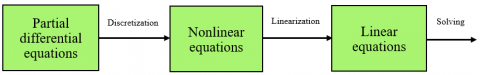
The established simulation model for CBM productivity describes the migration law of CBM and water in the coal reservoir. However, the partial differential equations in the model are nonlinear, and cannot be solved by analytical methods. Hence, these equations should be discretized and then solved by numerical methods. The solving process of the established CBM productivity model is explained in Figure 2.
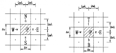
In FVM-based discretization, there are three optional formats: semi-implicit, fully implicit, and fully explicit [24, 25]. Here, the fully implicit format is selected for the FVM-based discretization of formulas (19) and (20). First, the solution domain was discretized as in Figure 3. In the 3D network, each control volume is a regular cuboid. Among them, node P has six neighboring nodes, namely, B, T, S, N, W and E.
Figure 2. The solving process of the established CBM productivity model
Figure 3. The 3D network of discretized solution domain
First, gas phase differential Eq. (19) was integrated on the control volume and time period:
$\int\limits_{t}^{t+\Delta t}{\int\limits_{b}^{t}{\int\limits_{s}^{n}{\int\limits_{w}^{e}{\frac{\partial }{\partial x}\left( \frac{\partial {{P}_{g}}}{\partial x} \right)\left( \frac{{{\rho }_{g}}{{K}_{rg}}{{K}_{x}}}{{{\mu }_{g}}} \right)}}}}dxdydzdt+\int\limits_{t}^{t+\Delta t}{\int\limits_{b}^{t}{\int\limits_{s}^{n}{\int\limits_{w}^{e}{\frac{\partial }{\partial y}\left( \frac{\partial {{P}_{g}}}{\partial y} \right)\left( \frac{{{\rho }_{g}}{{K}_{rg}}{{K}_{y}}}{{{\mu }_{g}}} \right)}}}}dxdydzdt+$
$\int\limits_{t}^{t+\Delta t}{\int\limits_{b}^{t}{\int\limits_{s}^{n}{\int\limits_{w}^{e}{\frac{\partial }{\partial z}\left( \frac{\partial {{P}_{g}}}{\partial z} \right)\left( \frac{{{\rho }_{g}}{{K}_{rg}}{{K}_{z}}}{{{\mu }_{g}}} \right)}}}}dxdydzdt-\int\limits_{t}^{t+\Delta t}{\int\limits_{b}^{t}{\int\limits_{s}^{n}{\int\limits_{w}^{e}{\frac{\partial }{\partial z}\left( \frac{{{\rho }_{g}}^{2}{{K}_{rg}}{{K}_{z}}g}{{{\mu }_{g}}} \right)}}}}dxdydzdt+\int\limits_{t}^{t+\Delta t}{\int\limits_{b}^{t}{\int\limits_{s}^{n}{\int\limits_{w}^{e}{{{q}_{m}}}}}}dxdydzdt$
$\int\limits_{t}^{t+\Delta t}{\int\limits_{b}^{t}{\int\limits_{s}^{n}{\int\limits_{w}^{e}{{{q}_{g}}}}}}dxdydzdt\text{=}\int\limits_{t}^{t+\Delta t}{\int\limits_{b}^{t}{\int\limits_{s}^{n}{\int\limits_{w}^{e}{\frac{\partial }{\partial t}\left( \phi {{\rho }_{g}}{{S}_{g}} \right)}}}}dxdydzdt$ (21)
Then, water phase differential equation (20) was integrated on the control volume and time period:
$\int\limits_{t}^{t+\Delta t}{\int\limits_{b}^{t}{\int\limits_{s}^{n}{\int\limits_{w}^{e}{\frac{\partial }{\partial x}\left( \frac{\partial {{P}_{w}}}{\partial x} \right)\left( \frac{{{\rho }_{w}}{{K}_{rw}}{{K}_{x}}}{{{\mu }_{w}}} \right)}}}}dxdydzdt+\int\limits_{t}^{t+\Delta t}{\int\limits_{b}^{t}{\int\limits_{s}^{n}{\int\limits_{w}^{e}{\frac{\partial }{\partial y}\left( \frac{\partial {{P}_{w}}}{\partial y} \right)\left( \frac{{{\rho }_{w}}{{K}_{rw}}{{K}_{y}}}{{{\mu }_{w}}} \right)}}}}dxdydzdt$
$+\int\limits_{t}^{t+\Delta t}{\int\limits_{b}^{t}{\int\limits_{s}^{n}{\int\limits_{w}^{e}{\frac{\partial }{\partial z}\left( \frac{\partial {{P}_{w}}}{\partial z} \right)\left( \frac{{{\rho }_{w}}{{K}_{rw}}{{K}_{z}}}{{{\mu }_{w}}} \right)}}}}dxdydzdt-\int\limits_{t}^{t+\Delta t}{\int\limits_{b}^{t}{\int\limits_{s}^{n}{\int\limits_{w}^{e}{\frac{\partial }{\partial z}\left( \frac{{{\rho }_{w}}^{2}{{K}_{rw}}{{K}_{z}}g}{{{\mu }_{w}}} \right)}}}}dxdydzdt$
$\text{-}\int\limits_{t}^{t+\Delta t}{\int\limits_{b}^{t}{\int\limits_{s}^{n}{\int\limits_{w}^{e}{{{q}_{w}}}}}}dxdydzdt\text{=}\int\limits_{t}^{t+\Delta t}{\int\limits_{b}^{t}{\int\limits_{s}^{n}{\int\limits_{w}^{e}{\frac{\partial }{\partial t}\left( \phi {{\rho }_{w}}{{S}_{w}} \right)}}}}dxdydzdt$ (22)
Next, formulas (21) and (22) were discretized and combined into:
$\left\{ \begin{align} & {{a}_{P}}{{\left( {{P}_{g}} \right)}_{P}}+{{a}_{W}}{{\left( {{P}_{g}} \right)}_{W}}+{{a}_{E}}{{\left( {{P}_{g}} \right)}_{E}}+{{a}_{S}}{{\left( {{P}_{g}} \right)}_{S}}+{{a}_{N}}{{\left( {{P}_{g}} \right)}_{N}}+{{a}_{B}}{{\left( {{P}_{g}} \right)}_{B}}+{{a}_{T}}{{\left( {{P}_{g}} \right)}_{T}}+{{b}_{P}}{{\left( {{S}_{g}} \right)}_{P}}=c \\ & {{c}_{P}}{{\left( {{P}_{w}} \right)}_{P}}+{{c}_{W}}{{\left( {{P}_{w}} \right)}_{W}}+{{c}_{E}}{{\left( {{P}_{w}} \right)}_{E}}+{{c}_{S}}{{\left( {{P}_{w}} \right)}_{S}}+{{c}_{N}}{{\left( {{P}_{w}} \right)}_{N}}+{{c}_{B}}{{\left( {{P}_{w}} \right)}_{B}}+{{c}_{T}}{{\left( {{P}_{w}} \right)}_{T}}+{{d}_{P}}{{\left( {{S}_{w}} \right)}_{P}}=e \\ \end{align} \right.$ (23)
${{a}_{P}}\text{=}-\frac{{{\left( \frac{{{\rho }_{g}}{{K}_{rg}}{{K}_{x}}}{{{\mu }_{g}}} \right)}_{P}}}{\frac{\Delta x}{\Delta y\Delta z}}-\frac{{{\left( \frac{{{\rho }_{g}}{{K}_{rg}}{{K}_{y}}}{{{\mu }_{g}}} \right)}_{P}}}{\frac{\Delta y}{\Delta x\Delta z}}-\frac{{{\left( \frac{{{\rho }_{g}}{{K}_{rg}}{{K}_{z}}}{{{\mu }_{g}}} \right)}_{P}}}{\frac{\Delta z}{\Delta x\Delta y}}-\frac{{{\left( \frac{{{\rho }_{g}}{{K}_{rg}}{{K}_{x}}}{{{\mu }_{g}}} \right)}_{W}}+{{\left( \frac{{{\rho }_{g}}{{K}_{rg}}{{K}_{x}}}{{{\mu }_{g}}} \right)}_{E}}}{\frac{2\Delta x}{\Delta y\Delta z}}$
$-\frac{{{\left( \frac{{{\rho }_{g}}{{K}_{rg}}{{K}_{y}}}{{{\mu }_{g}}} \right)}_{S}}+{{\left( \frac{{{\rho }_{g}}{{K}_{rg}}{{K}_{y}}}{{{\mu }_{g}}} \right)}_{N}}}{\frac{2\Delta y}{\Delta x\Delta z}}-\frac{{{\left( \frac{{{\rho }_{g}}{{K}_{rg}}{{K}_{z}}}{{{\mu }_{g}}} \right)}_{B}}+{{\left( \frac{{{\rho }_{g}}{{K}_{rg}}{{K}_{z}}}{{{\mu }_{g}}} \right)}_{T}}}{\frac{2\Delta z}{\Delta x\Delta y}}-{{\left( \frac{\pi h{{K}_{rg}}K{{\rho }_{g}}\Delta x\Delta y\Delta z}{{{\mu }_{g}}(\ln \frac{{{r}_{e}}}{{{r}_{w}}}+s)} \right)}_{P}}-{{\left[ \frac{G{{V}_{e}}\Delta x\Delta y\Delta z}{2\tau } \right]}_{P}}$ (24)
${{a}_{W}}=\frac{{{\left( \frac{{{\rho }_{g}}{{K}_{rg}}{{K}_{x}}}{{{\mu }_{g}}} \right)}_{P}}+{{\left( \frac{{{\rho }_{g}}{{K}_{rg}}{{K}_{x}}}{{{\mu }_{g}}} \right)}_{W}}}{\frac{2\Delta x}{\Delta y\Delta z}}\,\,\,\, , {{a}_{E}}=\frac{{{\left( \frac{{{\rho }_{g}}{{K}_{rg}}{{K}_{x}}}{{{\mu }_{g}}} \right)}_{P}}+{{\left( \frac{{{\rho }_{g}}{{K}_{rg}}{{K}_{x}}}{{{\mu }_{g}}} \right)}_{E}}}{\frac{2\Delta x}{\Delta y\Delta z}}$ (25)
${{a}_{S}}=\frac{{{\left( \frac{{{\rho }_{g}}{{K}_{rg}}{{K}_{y}}}{{{\mu }_{g}}} \right)}_{P}}+{{\left( \frac{{{\rho }_{g}}{{K}_{rg}}{{K}_{y}}}{{{\mu }_{g}}} \right)}_{S}}}{\frac{2\Delta y}{\Delta x\Delta z}}, {{a}_{N}}=\frac{{{\left( \frac{{{\rho }_{g}}{{K}_{rg}}{{K}_{y}}}{{{\mu }_{g}}} \right)}_{P}}+{{\left( \frac{{{\rho }_{g}}{{K}_{rg}}{{K}_{y}}}{{{\mu }_{g}}} \right)}_{N}}}{\frac{2\Delta y}{\Delta x\Delta z}}$ (26)
${{a}_{B}}=\frac{{{\left( \frac{{{\rho }_{g}}{{K}_{rg}}{{K}_{y}}}{{{\mu }_{g}}} \right)}_{P}}+{{\left( \frac{{{\rho }_{g}}{{K}_{rg}}{{K}_{z}}}{{{\mu }_{g}}} \right)}_{B}}}{\frac{2\Delta z}{\Delta x\Delta y}}, {{a}_{T}}=\frac{{{\left( \frac{{{\rho }_{g}}{{K}_{rg}}{{K}_{z}}}{{{\mu }_{g}}} \right)}_{P}}+{{\left( \frac{{{\rho }_{g}}{{K}_{rg}}{{K}_{z}}}{{{\mu }_{g}}} \right)}_{T}}}{\frac{2\Delta z}{\Delta x\Delta y}}$ (27)
$c=\frac{{{\left( \frac{{{\rho }_{g}}^{2}{{K}_{rg}}{{K}_{z}}g}{{{\mu }_{g}}} \right)}_{T}}-{{\left( \frac{{{\rho }_{g}}^{2}{{K}_{rg}}{{K}_{z}}g}{{{\mu }_{g}}} \right)}_{B}}}{2}\Delta x\Delta y-{{\left[ \frac{\pi h{{K}_{rg}}K{{\rho }_{g}}\Delta x\Delta y\Delta z}{{{\mu }_{g}}(\ln \frac{{{r}_{e}}}{{{r}_{w}}}+s)}{{P}_{wfg}} \right]}_{P}}+\left[ \frac{\pi h{{K}_{rg}}K{{\rho }_{g}}\Delta x\Delta y\Delta z}{{{\mu }_{g}}(\ln \frac{{{r}_{e}}}{{{r}_{w}}}+s)}({{P}_{g}}-{{P}_{wfg}}) \right]_{P}^{0}$
$-{{\left[ \frac{G{{V}_{m}}}{2\tau }\Delta x\Delta y\Delta z \right]}_{P}}-\left[ \frac{G\left[ {{V}_{m}}-{{V}_{e}}({{P}_{g}}) \right]\Delta x\Delta y\Delta z}{2\tau } \right]_{P}^{0}-\left( \phi {{\rho }_{g}}{{S}_{g}} \right)_{P}^{0}\frac{\Delta x\Delta y\Delta z}{\Delta t}$ (28)
${{b}_{P}}=-{{\left( \phi {{\rho }_{g}} \right)}_{P}}\frac{\Delta x\Delta y\Delta z}{\Delta t}$ (29)
${{c}_{P}}\text{=}-\frac{{{\left( \frac{{{\rho }_{w}}{{K}_{rw}}{{K}_{x}}}{{{\mu }_{w}}} \right)}_{P}}}{\frac{\Delta x}{\Delta y\Delta z}}-\frac{{{\left( \frac{{{\rho }_{w}}{{K}_{rw}}{{K}_{y}}}{{{\mu }_{w}}} \right)}_{P}}}{\frac{\Delta y}{\Delta x\Delta z}}-\frac{{{\left( \frac{{{\rho }_{w}}{{K}_{rw}}{{K}_{z}}}{{{\mu }_{w}}} \right)}_{P}}}{\frac{\Delta z}{\Delta x\Delta y}}-\frac{{{\left( \frac{{{\rho }_{w}}{{K}_{rw}}{{K}_{x}}}{{{\mu }_{w}}} \right)}_{W}}+{{\left( \frac{{{\rho }_{w}}{{K}_{rw}}{{K}_{x}}}{{{\mu }_{w}}} \right)}_{E}}}{\frac{2\Delta x}{\Delta y\Delta z}}$
$-\frac{{{\left( \frac{{{\rho }_{w}}{{K}_{rw}}{{K}_{y}}}{{{\mu }_{w}}} \right)}_{S}}+{{\left( \frac{{{\rho }_{w}}{{K}_{rw}}{{K}_{y}}}{{{\mu }_{w}}} \right)}_{N}}}{\frac{2\Delta y}{\Delta x\Delta z}}-\frac{{{\left( \frac{{{\rho }_{w}}{{K}_{rw}}{{K}_{z}}}{{{\mu }_{w}}} \right)}_{B}}+{{\left( \frac{{{\rho }_{w}}{{K}_{rw}}{{K}_{z}}}{{{\mu }_{w}}} \right)}_{T}}}{\frac{2\Delta z}{\Delta x\Delta y}}-{{\left( \frac{\pi h{{K}_{rw}}K{{\rho }_{w}}\Delta x\Delta y\Delta z}{{{\mu }_{w}}(\ln \frac{{{r}_{e}}}{{{r}_{w}}}+s)} \right)}_{P}}$ (30)
${{c}_{W}}=-\frac{{{\left( \frac{{{\rho }_{w}}{{K}_{rw}}{{K}_{x}}}{{{\mu }_{w}}} \right)}_{P}}+{{\left( \frac{{{\rho }_{w}}{{K}_{rw}}{{K}_{x}}}{{{\mu }_{w}}} \right)}_{W}}}{2\frac{\Delta x}{\Delta y\Delta z}}, {{c}_{E}}=\frac{{{\left( \frac{{{\rho }_{w}}{{K}_{rw}}{{K}_{x}}}{{{\mu }_{w}}} \right)}_{P}}+{{\left( \frac{{{\rho }_{w}}{{K}_{rw}}{{K}_{x}}}{{{\mu }_{w}}} \right)}_{E}}}{2\frac{\Delta x}{\Delta y\Delta z}}$ (31)
${{c}_{S}}=-\frac{{{\left( \frac{{{\rho }_{w}}{{K}_{rw}}{{K}_{y}}}{{{\mu }_{w}}} \right)}_{P}}+{{\left( \frac{{{\rho }_{w}}{{K}_{rw}}{{K}_{y}}}{{{\mu }_{w}}} \right)}_{S}}}{2\frac{\Delta y}{\Delta x\Delta z}}, {{c}_{N}}=\frac{{{\left( \frac{{{\rho }_{w}}{{K}_{rw}}{{K}_{y}}}{{{\mu }_{w}}} \right)}_{P}}+{{\left( \frac{{{\rho }_{w}}{{K}_{rw}}{{K}_{y}}}{{{\mu }_{w}}} \right)}_{N}}}{2\frac{\Delta y}{\Delta x\Delta z}}$ (32)
${{c}_{T}}=\frac{{{\left( \frac{{{\rho }_{w}}{{K}_{rw}}{{K}_{z}}}{{{\mu }_{w}}} \right)}_{P}}+{{\left( \frac{{{\rho }_{w}}{{K}_{rw}}{{K}_{z}}}{{{\mu }_{w}}} \right)}_{T}}}{2\frac{\Delta z}{\Delta x\Delta y}}, {{c}_{B}}=\frac{{{\left( \frac{{{\rho }_{w}}{{K}_{rw}}{{K}_{z}}}{{{\mu }_{w}}} \right)}_{P}}+{{\left( \frac{{{\rho }_{w}}{{K}_{rw}}{{K}_{z}}}{{{\mu }_{w}}} \right)}_{B}}}{2\frac{\Delta z}{\Delta x\Delta y}}$ (33)
$e=\frac{{{\left( \frac{{{\rho }_{w}}^{2}{{K}_{rw}}{{K}_{z}}g}{{{\mu }_{w}}} \right)}_{T}}-{{\left( \frac{{{\rho }_{w}}^{2}{{K}_{rw}}{{K}_{z}}g}{{{\mu }_{w}}} \right)}_{B}}}{2}\Delta x\Delta y-{{\left[ \frac{\pi h{{K}_{rw}}K{{\rho }_{w}}\Delta x\Delta y\Delta z}{{{\mu }_{w}}(\ln \frac{{{r}_{e}}}{{{r}_{w}}}+s)}\left( {{P}_{wfw}} \right) \right]}_{P}}$
$+\left[ \frac{\pi h{{K}_{rw}}K{{\rho }_{w}}\Delta x\Delta y\Delta z}{{{\mu }_{w}}(\ln \frac{{{r}_{e}}}{{{r}_{w}}}+s)}({{P}_{w}}-{{P}_{wfw}}) \right]_{P}^{0}-\left( \phi {{\rho }_{w}}{{S}_{w}} \right)_{P}^{0}\frac{\Delta x\Delta y\Delta z}{\Delta t}$ (34)
${{d}_{P}}=-{{\left( \phi {{\rho }_{w}} \right)}_{P}}\frac{\Delta x\Delta y\Delta z}{\Delta t}$ (35)
Finally, equation set (23) was integrated with the capillary force Eq. (9) and the saturation of methane in water equation (10) for solution.
3.3 Processing of boundary conditions
Before processing boundary conditions, it should be noted that, in the 3D network of the discretized solution domain, unit P corresponds to unit i, and W, E, N, S, B and T correspond to unit i-1, i+1, j+1, j-1, k-1 and k+1, respectively.
(1) Processing of outer boundary conditions
Each grid is represented by its center node. A row of virtual grids was set next to the boundary grids to process the corresponding outer boundary condition. The saturation and pressure on each boundary are known. The saturation and pressure of each virtual grid could be determined through linear interpolation. If the boundary is closed, the saturation and fluid potential of a virtual grid were assumed as equal to those of the adjacent boundary grid.
(2) Processing inner boundary conditions
To process diffusion and desorption terms, the methane content $C_{i, j, k}^{k}$ and $P_{g i, j, k}^{k}$ at grid (i,j,k) were directly substituted into the Fick’s first law of diffusion and Langmuir’s model on isotherm adsorption for calculation. The well points, e.g. the gas well or water well on grid (i,j,k), were processed by two different methods: if the downhole flow pressure is known, the equivalent supply radius was substituted into the equation of the grid; if the output $q_{w i, j, k}$ or $q_{g i, j, k}$ is known, the output was directly added to the equation of the grid.
3.4 Solving the CBM migration model
The Fluent software was adopted to compute the CBM migration, which belongs to the category of fluid mechanics. As a popular tool for fluid calculation, the software applies to various types of seepages, whether linear or nonlinear, and supports multiple types of grids, ranging from discontinuous grids, sliding grids, dynamic/deformed grids to mixed grids. With the aid of Fluent, the user can easily mesh complex areas into structural grids and unstructured grids, and roughen or refine the grids locally or globally according to the solutions scale, efficiency and accuracy. In addition, the software offers various solution-based grid adaptive, and dynamic adaptive techniques. Even if the flow area has a large gradient, the user can still obtain high-precision solutions of the flow field, using the adaptive grids provided by the software.
4.1 Preset parameters
This section applies the established model for simualte the CBM produtivity of a single well in the CBM development zone in the south of Qinshui Basin, Shanxi Province, China. The basic data cover reservoir features (coal quality, pore permeability, adsorption, reservoir temperature, reservoir pressure, etc.), reservoir space (coalbed thickness, geological structure, buried depth, etc.), well (well structure, in coefficient, etc.), pilot production (gas output, water ouput, downhole flow pressure, working fluid level, etc.), and the pressure, volume and temperature (PVT) of the fluid. The basic data were mainly collected through geological survey and development test, and supplemented by the geological work of mines.
Table 1 provides the main coal reservoir parameters adopted for example analysis.
Table 1. The reservoir parameters of the study area
|
Parameter |
Gas content m3·t-1 |
Water saturation % |
Coal thickness m |
Reservoir pressure MPa |
pL MPa |
VL m3·t-1 |
Gas saturation % |
Initial permeability mD |
|
Mean values |
17.65 |
1.49 |
5.75 |
3.36 |
3.12 |
46.34 |
76 |
0.76 |
4.2 FVM-based simulation of CBM productivity
4.2.1 Fitting of CBM well production curve
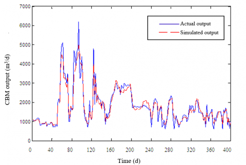
The drainage and production curves of a CBM well from February 12, 2013 to March 17, 2014 were simulated. The grids of the simulation area are shown in Figure 4. It is assumed that the gas only contains methane. Neither the matrix shrinkage effect of reservoir permeability nor the heterogeneity of the reservoir was considered. Then, the FVM-based simulation model was applied to simulate the single-well productivity in the simulation area and fit the historical production curve. Based on the simulation, the reservoir parameters were adjusted and corrected continuously, making them more realistic. Through multiple fittings, the obtained curves of the historical gas and water outputs are shown in Figures 5 and 6.
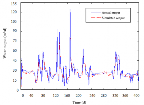
As shown in Figures 5 and 6, the simulated curves approximated the actual gas and water outputs well, and basically agree with the overall trend of the historical drainage and production curves of the CBM well. The excellent results are attributable to the adjustment and correction of some fitting parameters. Table 2 lists the parameters to be adjusted and the fitted values. These values will be combined with the data in Table 1 for productivity prediction.
Figure 4. The grids of the simulation area
Figure 5. Fitted curve of the historical gas output of the single CBM well
Figure 6. Fitted curve of the historical water output of the single CBM well
Table 2. Adjustment of fitting parameters
|
Parameter |
Reservoir permeability /mD |
Cleat porosity /% |
Skin coefficient |
Gas content / m3·t-1 |
|
Initial value |
0.76 |
5.19 |
1.7 |
17.65 |
|
Fitted value |
1.1 |
1.7 |
1.3 |
21.6 |
4.2.2 Prediction of the productivity of the CBM well
To maximize the production efficiency of the CBM well, the development measures should be adjusted and corrected continuously. This requires clear understanding of how each stage of gas production affects the CBM productivity. For this purpose, our FVM-based model was adopted to predict the productivity of the CBM well, and the simulated results were compared with the data obtained through well testing and sample test.
During the simulation, the daily gas output and daily water output of a single CBM well were predicted for the 500 production days after June 22, 2013, revealing the change trends. In the selected prediction curves, the gas output gradually decreased from the initial level of around 4,000m3/d, while the water output plunged from the initial level of 120m3/d to the final level of about 20m3/d. The reservoir parameters were adjusted and corrected before the prediction. The productivity curves predicted by our model are shown in Figure 7.
Figure 7. Predicted productivity of the CBM well
As shown in Figure 7, the daily gas output of the CBM well declined continuously since June, 2013, and did not stabilize after 1.5 years of drainage and production; the daily water output of the CBM well plunged unceasingly since June, 2013, and basically stabilized at 20m3/d after quite a few months. Therefore, the FVM-based model has successfully predicted the change trend of the productivity of the CBM well, revealing the high reliability and confidence of the model.
There are many reports on the influencing factors of the single-well productivity in the south of Qinshui Basin. It is generally believed that the daily gas output of a single CBM well is mainly affected by the reservoir pressure, permeability, gas content and cleat porosity. Several other factors also have varied degrees of impact on the single-well productivity, namely, maximum initial water output, gas saturation, fracture half-length, skin coefficient, desorption time, and buried depth.
4.2.3 Sensitivity analysis of reservoir parameters
The single-well productivity may be affected by various reservoir parameters. Here, three major reservoir parameters, i.e. gas content, maximum initial water output and fracture half-length, are selected to analyze the sensitivity of single-well productivity to each of them. The parameter values were set rationally within the intervals determined by experiments or measured data, and adjusted across the corresponding interval. In addition, the other parameters were kept constant, when one parameter was subjected to sensitivity analysis.
(1) Influence of gas content
The gas contents of 10m3, 12m3, 14m3, 16m3 and 18m3 were imported to our model in turn. According to the simulated results in Figure 8, the gas output of the CBM well increased with the gas content. Without changing the other parameters, the gas output exhibited a linear growth, as the gas content increased at the step length of 2m3. As the gas content increased from 10m3 to 18m3, the gas output surged up from 200m3 to the peak of 1,500m3. The pre-peak curve was very steep and the peak lasted for a very short time, indicating that gas content has an obvious influence on the gas output of the CBM well. The gas content also affects the time point of the plateau production: the higher the gas content, the earlier the plateau production.
(2) Influence of maximum initial water output
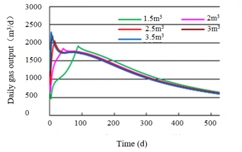
The maximum initial water outputs of 1.5m3, 2m3, 2.5m3, 3m3 and 3.5m3 were inputted into our model in turn. According to the simulated results in Figure 9, in the early phase of development, the gas output increased with the maximum initial water output; the higher the maximum initial water output, the faster it is to reach the peak gas output. The maximum initial water output mainly influenced the gas output before it reached the peak level. As the maximum initial water output grew from 1. 5m3 to 3.5m3, the peak gas output climbed from 1,700m3 to 2,300m3. The higher the maximum initial water output, the earlier the peak gas output appears. The inverse is also true. Hence, the maximum initial water output has an obvious influence on the time point of the peak gas output.
(3) Influence of fracture half-length
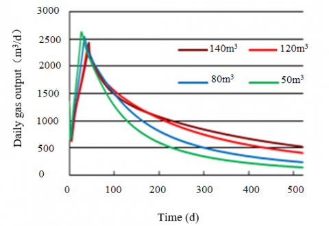
The fracture half-lengths of 50m, 80m, 120m and 140m were imported to our model in turn. According to the simulated results in Figure 10, the fracture half-length mainly influenced the gas output after it reached the peak level. As the fracture half-length grew from 50m to 140m, the gas output increased accordingly. Before the peak, the gas output curve was extremely steep, indicating that the fracture half-length has a major impact on gas output. The gas output could be improved significantly when the fractured half-length falls into a certain interval, i.e. there exists an optimal fractured half-length for fracturing stimulation. The most effective way to increase the fracture half-length is hydraulic fracturing. Of course, the gas output is not necessarily better with the growth in the fracture half-length. The interference between adjacent wells must be considered to determine the optimal fracture half-length.
From Figures 8-10, it can be seen that gas content, maximum initial water output and fracture half-length all have an obvious impact on the gas output of the CBM well.
Figure 8. Influence of gas contents on gas output
Figure 9. Influence of maximum initial water outputs on gas output
Figure 10. Influence of fracture half-lengths on gas output
This paper proposes a simulation model for CBM productivity based on the FVM, and uses the model to predict and fit the historical productivity of a single well in a simulation area. Based on the simulated results, the reservoir parameters were adjusted and corrected continuously, making them more realistic. Then, the historical gas and water output curves were fitted with our model, and the simulated curves approximated the actual gas and water outputs well. Next, the change trends of gas and water outputs in the CBM well were predicted in a correct manner. Finally, the sensitivities of gas well productivity to three main reservoir parameters were analyzed in details. The example analysis shows that our model can be promoted in CBM exploration and development.
This work is supported by National Natural Science Foundation of China (Grant No.: 40972207), National Science and Technology Major Project (Grant No.: 2011ZX05034-005), and Chinese Postdoctoral Science Foundation (Grant No.: 102081902).
[1] Zheng, D.Z., Zhao, D.F. (2018). Research on development policy of coalbed methane industry in China's coal mining areas. Coal Economic Research, 38(11): 60-65. https://doi.org/10.13202/j.cnki.cer.2018.11.011
[2] Sarhosis, V., Jaya, A.A., Thomas, H.R. (2016). Economic modelling for coal bed methane production and electricity generation from deep virgin coal seams. Energy, 107: 580-594. https://doi.org/10.1016/j.energy.2016.04.056
[3] Ma, T., Rutqvist, J., Oldenburg, C.M., Liu, W. (2017). Coupled thermal–hydrological–mechanical modeling of CO2-enhanced coalbed methane recovery. International Journal of Coal Geology, 179: 81-91. https://doi.org/10.1016/j.coal.2017.05.013
[4] Ziarani, A.S., Aguilera, R., Clarkson, C.R. (2011). Investigating the effect of sorption time on coalbed methane recovery through numerical simulation. Fuel, 90(7): 2428-2444. https://doi.org/10.1016/j.fuel.2011.03.018
[5] Lie, K.A., Møyner, O., Natvig, J.R. (2017). Use of multiple multiscale operators to accelerate simulation of complex geomodels. SPE Journal, 22(06): 1-929. https://doi.org/10.2118/182701-PA
[6] Reeves, S., Pekot, L. (2001). Advanced reservoir modeling in desorption-controlled reservoirs. In SPE Rocky Mountain Petroleum Technology Conference. Society of Petroleum Engineers.
[7] Lv, S.J., Wang, J.C. (2006). Application of finite volume method in numerical simulation of soil water movement. Science & Technology Information, 34:185-186. https://doi.org/10.3969/j.issn.1672-3791.2006.34.151
[8] Vishal, V., Singh, T.N., Ranjith, P.G. (2015). Influence of sorption time in CO2-ECBM process in Indian coals using coupled numerical simulation. Fuel, 139: 51-58. https://doi.org/10.1016/j.fuel.2014.08.009
[9] Taheri, A., Sereshki, F., Ardejani, F.D., Mirzaghorbanali, A. (2017). Simulation of macerals effects on methane emission during gas drainage in coal mines. Fuel, 210: 659-665. https://doi.org/10.1016/j.fuel.2017.08.081
[10] Hower, T.L. (2003). Coalbed methane reservoir simulation: An evolving science. In SPE Annual Technical Conference and Exhibition. Society of Petroleum Engineers. https://doi.org/10.2118/84424-MS
[11] Vilarrasa, V., Rutqvist, J. (2017). Thermal effects on geologic carbon storage. Earth-Science Reviews, 165: 245-256. https://doi.org/10.1016/j.earscirev.2016.12.011
[12] Jiang, W., Wu, C., Wang, Q., Xiao, Z., Liu, Y. (2016). Interlayer interference mechanism of multi-seam drainage in a CBM well: An example from Zhucang syncline. International Journal of Mining Science and Technology, 26(6): 1101-1108. https://doi.org/10.1016/j.ijmst.2016.09.020
[13] Kim, S., Ko, D., Mun, J., Kim, T.H., Kim, J. (2018). Techno-economic evaluation of gas separation processes for long-term operation of CO2 injected enhanced coalbed methane (ECBM). Korean Journal of Chemical Engineering, 35(4): 941-955. https://doi.org/10.1007/s11814-017-0261-4
[14] Lee, S., Yun, S., Kim, J.K. (2019). Development of novel sub-ambient membrane systems for energy-efficient post-combustion CO2 capture. Applied Energy, 238: 1060-1073. https://doi.org/10.1016/j.apenergy.2019.01.130
[15] Mallick, N., Prabu, V. (2017). Energy analysis on Coalbed Methane (CBM) coupled power systems. Journal of CO2 Utilization, 19: 16-27. https://doi.org/10.1016/j.jcou.2017.02.012
[16] Le, T.D., Murad, M.A., Pereira, P.A. (2017). A new matrix/fracture multiscale coupled model for flow in shale-gas reservoirs. SPE Journal, 22(01): 265-288. https://doi.org/10.2118/181750-PA
[17] Li, B., Zhao, L.C., Wang, L., Liu, C., McAdam, K.G., Wang, B. (2016). Gas-phase pressure and flow velocity fields inside a burning cigarette during a puff. Thermochimica Acta, 623: 22-28. https://doi.org/10.1016/j.tca.2015.11.006
[18] Liu, P., Qin, Y., Liu, S., Hao, Y. (2018). Non-linear gas desorption and transport behavior in coal matrix: Experiments and numerical modeling. Fuel, 214: 1-13. https://doi.org/10.1016/j.fuel.2017.10.120
[19] Qu, H., Liu, J., Pan, Z., Peng, Y., Zhou, F. (2017). Simulation of coal permeability under non-isothermal CO2 injection. International Journal of Oil, Gas and Coal Technology, 15(2): 190-215. https://doi.org/10.1504/IJOGCT.2017.084317
[20] Ewing, R., Lazarov, R., Lin, Y. (2000). Finite volume element approximations of nonlocal reactive flows in porous media. Numerical Methods for Partial Differential Equations: An International Journal, 16(3): 285-311. https://doi.org/10.1002/(SICI)1098-2426(200005)16:3<285::AID-NUM2>3.0.CO;2-3
[21] Wang, Q., Ren, Y.X. (2015). An accurate and robust finite volume scheme based on the spline interpolation for solving the Euler and Navier–Stokes equations on non-uniform curvilinear grids. Journal of Computational Physics, 284: 648-667. https://doi.org/10.1016/j.jcp.2014.12.050
[22] Yu, C., Duan, J. (2012). Two-dimensional depth-averaged finite volume model for unsteady turbulent flow. Journal of Hydraulic Research, 50(6): 599-611. https://doi.org/10.1080/00221686.2012.730556
[23] Zheng, C. (2016). Sparse equidistribution of unipotent orbits in finite-volume quotients of PSL (2, R). (Doctoral dissertation, The Ohio State University), 10(2): 1-21. http://rave.ohiolink.edu/etdc/view?acc_num=osu1467320625
[24] Ghadimi, M., Farshchi, M. (2012). Fourth order compact finite volume scheme on nonuniform grids with multi-blocking. Computers & Fluids, 56: 1-16. https://doi.org/10.1016/j.compfluid.2011.11.007
[25] Buenger, C.D., Zheng, C. (2017). Non-divergence of unipotent flows on quotients of rank-one semisimple groups. Ergodic Theory and Dynamical Systems, 37(1): 103-128. https://doi.org/10.1017/etds.2015.43