OPEN ACCESS
This paper investigates the water-oil displacement flow in a downward inclined pipe, which is applied in practice in the chemical and oil industries. The computational fluid dynamics (CFD) method was applied in the simulation of the displacement process. The simulation procedure was performed in a structured grid with refinement near the boundary, and the Volume of Fluid method was used as the multiphase model. Three flow patterns were obtained and the simulated data were favorably matched with the experiment results. Further efforts were made where parametric studies were concerned, including the effects of pipe diameter, inclination angle, and water inlet velocity on the displacement process. It was concluded that the displacement efficiency can be improved by increasing the water inlet velocity, and the increasing pipe inclination angle may lead to the instability of the interface.
immiscible displacement, residual layer, interface instability, numerical simulation
Displacement flow is a technique commonly used in industrial applications, such as the removal of liquid products remaining in the pipeline in the chemical industry, and secondary oil recovery in the oil industry. Many factors, such as the physical and chemical properties of displaced and displacing fluids, entry and boundary conditions, and gravity all contribute to the variability and complexity of the displacement flows. In order to achieve high-quality displacement flows, the degree and extent of the mixing between the fluids are critical. With the purpose of minimizing the mixing region, it is desirable to achieve a fundamental understanding of the mechanism and characteristics of the displacement process.
Numerous studies have focused on both miscible and immiscible displacement flows. Flow pattern transition, interface instability, and displacement efficiency are the focus of many research papers. The miscible displacement flows are always associated with molecular diffusion [1]. For the miscible displacements of a more viscous fluid by a less viscous one, in most cases the less viscous fluid may finger into the more viscous one, thus forming a two or three-layer flow structure [2-3]. In recent decades, miscible displacement in porous media and low Reynolds numbers have received considerable attention [4-6]. For miscible displacement flows in high Peclet numbers, the diffusion effect between fluids can be neglected and the fluids can be regarded as immiscible [7].
Compared with miscible displacements, the immiscible displacement flows have almost no diffusion effect between phases. The displacement of yield stress fluids such as waxy crude oils has been studied analytically [8] and numerically [9]. The static wall layers of the yield stress fluids can be attached to the pipe wall in such displacement flows [10]. In particular, if the displacement procedure proceeds with balanced axial buoyancy force and viscous force in a downward pipe, the lighter displaced fluid may remain stationary in the upper pipe section as observed in previous experiments [11]. Once the stationary residual layers are formed, the efficiency of the displacement will be greatly affected. In industrial applications the immiscible displacement flows are also considered, including the process of trapped water displacement using oil flooding [12], and the residual oil displacement in a sinusoidal channel [13].
Numerical methods have been utilized to investigate the displacement flow. The immiscible displacement of yoghurt by water has been studied using the CFD method [14]. It is indicated that the RNG k-ε with enhanced wall treatment and the k-ω turbulence models are efficient for predicting the immiscible displacement flows with laminar and turbulent flows coexisting. The miscible displacement with density gradient is simulated [15], and it is proved that the increasing density ratio and Froude number enhance the instability of the displacement flow. The double diffusive effects in the displacement flow are also studied [16], and the results show that double-diffusive effects destabilize the displacement flow.
Despite a large number of studies carried out on displacement flows and water-oil two-phase flows, few studies concentrate on the water-oil displacement flow in inclined pipes, which is a special case of the Newtonian immiscible displacement flows. In the present study, experiments are initially performed in a downward inclined pipe. Then the experimental results are verified with the predictions of the CFD simulations. Finally, parametric studies are implemented to give detailed flow hydrodynamics of the water-oil displacement.
2.1 Model geometry
The CFD simulation of water-oil displacement in inclined pipe sections is considered, and the model geometry is shown in Figure 19(a). The pipe section is downward inclined with the inclination angle α varying from 0º to 30º. The water is injected from upstream to displace the oil in the pipe. For data comparison, two cases with different pipe diameters, i.e. 0.015m and 0.02m, are considered respectively. In both cases the computation length L for the pipe is 0.6m. Moreover, the computational domain is separated into a water section and an oil section. The water section is set at 0≤z≤0.05m and is initially filled with water to avoid entry effects [17]. We have ensured that the computation pipe length is long enough so that the simulation results are insensitive to the computational length.
Figure 1. Schematic view of model geometry and generated mesh
2.2 Multiphase model
To track the interface between water and oil, the VOF method is selected as the multiphase model, due to the immiscibility of the fluids and the relatively well-defined interface of the flows. According to the VOF method, the volume fraction for each phase is calculated in each computational cell, and the fields for all variables and properties are shared by the phases. For a definite variable in each cell, the corresponding values for each phase depend on their volume fraction values. The momentum equation shared by each phase is solved throughout the computational domain, and the resulting velocity field is shared among the phases.
The surface tension effects and wall adhesion can be included in the VOF model [18]. The continuum surface force (CSF) model is used as the surface tension model in ANSYS Fluent and expressed as the pressure jump across the surface. The curvature of the surface is determined by the contact angle combined with the calculated surface normal one cell away from the wall. This curvature is used to adjust the body force term in the surface tension calculation [19].
2.3 Initial and boundary conditions
As mentioned above, the computational domain is divided into two sections, namely the water section and oil section. The water section and oil section are initially filled with water and oil, respectively. The fluids in the pipe are initially stationary at 21℃. The water velocity is specified at x=0. The boundary condition of the wall of the pipe is defined as no-slip and stationary.
3.1 Mesh for the geometric model
The meshing procedure for the geometric model has been carried out in ANSYS ICEM software. An O-type multi-block structured grid is used with refinement near the wall since the velocity field is sharply varied in the near-wall region and there oil layers are likely to be attached to the pipe wall. The cross-section view of the meshed model geometry for the pipe with an inner diameter of 0.02m is shown in Figure 1(b). The mesh generation strategy for a pipe with an inner diameter of 0.015m is the same as for one of 0.02m, but is different in grid densities. The mesh of the cross section is mapped along the length of the pipe.
To ensure the independence of the mesh, the volume fraction of the oil for the whole pipe is computed and compared under varying grid densities. Independent mesh tests are implemented for a pipe of d=0.015m and d=0.02m with constant inlet velocity of 0.6m/s and 0.45m/s respectively. Considering both computational efficiency and accuracy, the cell number 1099056 is chosen for d=0.015m and 121835 for d=0.02m.
3.2 Discretization methods
The pressure-implicit with splitting of operator (PISO) algorithm with neighbor correction, which can maintain a stable calculation with a larger time step and an under-relaxation factor for both momentum and pressure, is applied in the pressure-velocity coupling process [20]. The pressure staggering option (PRESTO) scheme is used for pressure interpolation. In addition, the geometric reconstruction interpolation scheme is used for discretization in volume fraction, with the purpose of obtaining the time-accurate transient behavior of the VOF solution. In order to discretize the momentum equation, the second order upwind method is adopted, while the scheme for transient formulation is first order implicit. The time step size is adjusted, and as a result the value of the global Courant number remains under 1 during the calculation process.
The displacement procedure was conducted in a 3.5m long, 15mm inner diameter downward glass pipe with a corresponding pipeline system loop. The pipe was connected to a hose pipe at both ends and was fixed on a steel frame that could be flexibly tilted to a specific inclination angle. A pressure water tank was used as a pressure source to avoid mechanical vibration from the water pump and supply relative stable inlet flow. A fluorescent yellow coloring agent which only dissolves in oil was added to diesel in order to distinguish the two phases and visualize the oil-water interface. The density of diesel, which was measured under 21℃, was 829.4 kg/m3 and the viscosity was 3.3mPa s with a diesel-water interfacial tension of 18.2 mN/m. Meanwhile, the density of the water was 998.3kg/m3, and the viscosity was 1.03mPa s.
The experiments were started by initially feeding the pipe with a high-speed oil flow by pumping from the oil tank to remove the air and water and fill the glass pipe with diesel oil. Then water was injected into the glass pipe as the displacing fluid with a needle valve regulating the imposed water flow rate. The degree of the valve was adjusted before the water injection and remained unchanged during the whole displacement process. The procedure continued until the flow reached a steady state. The superficial water flow rate was measured by two rotameters which were installed upstream of the glass pipe with different measuring ranges and with an accuracy of ±2%. The whole displacement process was recorded by a digital camera with 800fps. From the photographs captured, we could portray the concentration distribution of the oil phase and water phase and determine the frontal velocity as well as the interface height.
The simulations were performed under the conditions of different inlet velocities, pipe inclination angles, and pipe diameters within the experimental range. Initially the simulated data points are plotted in the flow pattern maps obtained from the experiments, and several experimental flow configurations are presented against the simulated results (as shown in Figure 2). The water is injected from the left margin. The flow configurations are divided into three categories, i.e. stationary residual layer, instantaneous displacement, and dispersed displacement. The stationary residual layer denotes the flow in which the oil layer remains stationary in the upper section of the pipe. As depicted in Figure 2, after the needle valve was opened, the water penetrated into the oil, and passed through the oil layer from underneath. Although the water continued to be injected, only part of the oil was displaced by the water flooding in. The remaining oil layer was still attached to the upper section and remained stationary until the end of the experiment. An instantaneous displacement occurs with increased water inlet velocity V0 when there is no stationary oil layer attached to the pipe wall. In this flow pattern, a few oil droplets would form in the frontal regime, and the water-oil interface tends to be waxy. A dispersed displacement is observed in high inlet water velocity. In this flow pattern, a large amount of oil droplets is produced in both the frontal regime and interface due to interface instability. It is revealed that a larger pipe diameter would lead to larger, critical speed for transitions. The simulated concentration distributions show favorable matching with experimental results. But the interface waviness is not precisely captured due to the constraints of the VOF method, which does not reconstruct the interface as a continuous chain [21]. It can be seen from Figure 2 that the increasing pipe inclination angle may lead to interface instability.
Figure 2. Comparison of simulations and photographs of flow configurations
The concentration contours of different oil flow patterns are presented in Figs. 3a-c. Figure 3(a) presents the variation in the cross-sectional concentration field of a stationary oil layer at frontal regimes. It is revealed that a two-layer structure is formed and the oil layer occupies the upper section of the pipe section. Near the frontal regime the water layer remains at the bottom of the pipe. A three-layer structure is formed in the cross-sectional view of the flow pattern of instantaneous displacement and dispersed displacement, as shown in Figs. 3(b) and Figure 3(c) and it can be concluded that the interface waves and oil droplets are three-dimensional, which is consistent with the experiment.
Figure 3. Concentration contours of oil at frontal regimes of different flow patterns
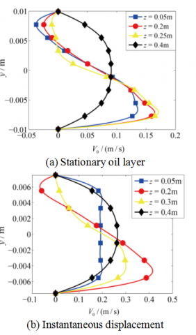
Figure 4. Velocity profile along y axial direction of different flow configurations
The velocity profile along the y axial direction at particular flow configurations is presented in Figs. 4(a)-(b), which represent the flow patterns of the stationary residual layer and instantaneous displacement, respectively. The flow configurations are the same as in Figure 2. In the flow pattern of the stationary residual layer (Figure 4(a)), the flow is usually laminar. As a result of the dominant buoyant effect, there is back flow in the upper region of the pipe section upstream of the leading front, which is in the opposite direction against the mean flow. As the Reynolds number increases, the flow pattern converts to instantaneous displacement (Figure 4(b)). In this flow pattern, back flow occurs only in the oil region. In the oil region the flow is laminar, while in the water region the flow is turbulent.
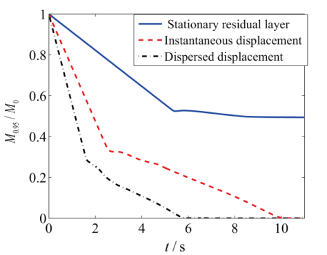
Figure 5 presents the variation in mass fraction of oil with the time of different flow patterns. As shown in Figure 5, before the leading front reaches the end of the computational domain, the mass fraction of oil linearly decreases with the time and the slope of the curve is related with the inlet water velocity. When the leading front reaches the computational domain, the slope of the curve decreases to a smaller value that varies according to different flow patterns. In the flow pattern of the stationary oil layer, the slope of the curve approximately decreases to zero while the corresponding mass fraction of oil is 0.49, which denotes that there is stationary oil remaining in the pipe. The mixing region, in which water penetrates into the oil, is much smaller when the flow pattern is dispersed than in instantaneous displacement. As can be seen, an increase in inlet water velocity can effectively reduce the mixing region between oil and water.
Figure 5. Variation in mass fraction of oil with time of different flow patterns
The CFD method has been applied in the simulation of water-oil displacement flow in downward inclined pipes. The simulation procedure was performed with different pipe diameters, pipe inclination angles, and water inlet velocities within the experimental range. The simulations are validated by the experimental results. From our present study, the following conclusions can be derived:
(1) Three flow patterns are identified, i.e. stationary residual layer, instantaneous displacement, and dispersed displacement. It is revealed that both pipe inclination and the Reynolds number influence the flow pattern transitions.
(2) In the flow pattern of the stationary oil layer, back flow occurs due to the buoyancy effect and the thickness of the oil layer is positively correlated with the pipe inclination angle. When the flow reaches a stable state, the oil layer remains stationary in the upper section of the pipe. But with increasing water inlet velocity, the thickness of the oil layer decreases and a flow transition may occur.
(3) It is inferred that the waviness of the interface may lead to a deviation between simulations and experimental results.
(4) It is revealed that the displacement efficiency can be improved by increasing the water inlet velocity, and an instability of the interface may occur with an increasing pipe inclination angle.
We thank the Department of Oil Supply Engineering for the support in the experimental design and setup.
[1] Taghavi S.M., Alba K., Seon T., Wielage-Burchard K., Martinez D.M., Frigaard I.A. (2012). Miscible displacement flows in near-horizontal ducts at low Atwood number, Journal of Fluid Mechanics, Vol. 696, No. 4, pp. 175-214. DOI: 10.1017/jfm.2012.26
[2] Sahu K.C., Ding H., Valluri P., Matar O.K. (2009). Linear stability analysis and numerical simulation of miscible two-layer channel flow, Physics of Fluids, Vol. 21, No. 4, pp. 65-517. DOI: 10.1063/1.3116285
[3] Feng F.P., Ai C., Xu H.S., Cui Z.H., Gao C.L. (2015). Research on the condition model of drilling fluid non-retention in eccentric annulus, International Journal of Heat and Technology, Vol. 33, No. 1, pp. 9-16.
[4] Droniou J., Talbot K.S. (2017). Analysis of miscible displacement through porous media with vanishing molecular diffusion and singular wells, Annales de l'Institut Henri Poincare (C) Non-Linear Analysis. DOI: 10.1016/j.anihpc.2017.02.002
[5] Chen F., Chen H. (2013). A BrokenP1-Nonconforming Finite Element Method for Incompressible Miscible Displacement Problem in Porous Media, ISRN Applied Mathematics, Vol. 2013, pp. 1-7. DOI: 10.1155/2013/498383
[6] Saffman P.G., Taylor G. (1988). The penetration of a fluid into a porous medium or Hele-Shaw cell containing a more viscous liquid, Dynamics of Curved Fronts, Vol. 245, No. 1242, pp. 155-174. DOI: 10.1016/B978-0-08-092523-3.50017-4
[7] Séon T., Hulin J.P., Salin D., Perrin B., Hinch E.J. (2005). Buoyancy driven miscible front dynamics in tilted tubes, Physics of Fluids, Vol. 17, No. 3, pp. 031702. DOI: 10.1063/1.1863332
[8] Frigaard I., Vinay G., Wachs A. (2007). Compressible displacement of waxy crude oils in long pipeline startup flows, Journal of Non-Newtonian Fluid Mechanics, vol. 147, No. 1, pp. 45-64. DOI: 10.1016/j.jnnfm.2007.07.002
[9] Redapangu P.R., Chandra Sahu K., Vanka S.P. (2012). A study of pressure-driven displacement flow of two immiscible liquids using a multiphase lattice Boltzmann approach, Physics of Fluids, Vol. 24, No. 10, pp. 102-110. DOI: 10.1063/1.4760257
[10] Allouche M., Frigaard I.A., Sona G. (2000). Static wall layers in the displacement of two visco-plastic fluids in a plane channel, Journal of Fluid Mechanics, Vol. 424, pp. 243-277. DOI: 10.1017/S0022112000001956
[11] Taghavi S.M., Séon T., Wielage-Burchard K., Martinez D.M., Frigaard I.A. (2011). Stationary residual layers in buoyant Newtonian displacement flows, Physics of Fluids, Vol. 23, pp. 044-105.
[12] Xu G.L., Zhang G.Z., Liu G., Ullmann A., Brauner N. (2011). Trapped water displacement from low sections of oil pipelines, International Journal of Multiphase Flow, Vol. 37, No. 1, pp. 1-11. DOI: 10.1016/j.ijmultiphaseflow.2010.09.003
[13] Otomo H., Fan H., Hazlett R., Li Y., Staroselsky I., Zhang R., Chen H. (2015). Simulation of residual oil displacement in a sinusoidal channel with the lattice Boltzmann method, Comptes Rendus Mécanique, vol. 343, No. 10-11, pp. 559-570. DOI: 10.1016/j.crme.2015.04.005
[14] Regner M., Henningsson M., Wiklund J., Östergren K., Trägårdh C. (2007). Predicting the displacement of yoghurt by water in a pipe using CFD, Chemical Engineering & Technology, Vol. 30, pp. 844-853.
[15] Sahu K.C., Ding H., Valluri P., Matar O.K. (2009). Pressure-driven miscible two-fluid channel flow with density gradients, Physics of Fluids, Vol. 21, No. 4, pp. 043603.
[16] Sahu K.C. (2013). Double diffusive effects on pressure-driven miscible channel flow: Influence of variable diffusivity, International Journal of Multiphase Flow, Vol. 55, pp. 24-31.
[17] Bhagat K.D., Tripathi M.K., Sahu K.C. (2016). Instability due to double-diffusive phenomenon in pressure-driven displacement flow of one fluid by another in an axisymmetric pipe, European Journal of Mechanics - B/Fluids, Vol. 55, pp. 63-70.
[18] Song H.J., Zhang W., Li Y.Q., Yang Z.Y., Ming A.B. (2016). Simulation of the vapor-liquid two-phase flow of evaporation and condensation, International Journal of Heat and Technology, Vol. 34, No. 4, pp. 663-670.
[19] Bhaskar K.U., Murthy Y.R., Raju M.R., Tiwari S., Srivastava J.K., Ramakrishnan N. (2007). CFD simulation and experimental validation studies on hydro cyclone, Minerals Engineering, Vol. 20, pp. 60-71.
[20] Inc A. (2013). ANSYS Fluent Theory Guide.
[21] Kaushik V.V.R., Ghosh S., Das G., Das P.K. (2012). CFD simulation of core annular flow through sudden contraction and expansion, Journal of Petroleum Science and Engineering, Vol. 86-87, pp. 153-164.