OPEN ACCESS
This article presents a numerical analysis of multi–phase flow with powerful swirling streams in a cylindrical separator equipped with two vortex generators in an attempt to predict the separation efficiency of an air–water mixture. New design of a cylindrical separator is introduced for air–water mixture. The mixture multiphase and large eddy simulation (LES) turbulence models were applied. Images that concern velocity field, pressure, and volume fraction ar
air separator, double vortex generator, turbulent, multi–phase, LES
Air is a source of problems in closed-circuit liquid circulation in HVAC (heating, ventilation and air conditioning) systems. The primary source of air is the dissolved gases in the makeup water to the system. There are a number of different types of devices available to remove air from HVAC system, including the basic expansion tank with a free air-water interface. However, in larger systems it is advisable to also use some other type of device such as air separator. One popular type of air elimination devices is the vortex air separator which generates a vortex inside the vessel that creates a low pressure zone in the center of the unit, causing air to bubble out of solution. The air then rises to top, where it is released through an automatic air vent. Application of these devices may be somewhat different for hot-water and chilled-water systems and also depends on the type of compression tank used [1].
In oil industry, the gas-liquid separation technology has been implemented long time ago based on gravity-driven technology that uses a costly bulky conventional separator. An alternative to the conventional gravity-based separator is conventional vessel-type separator that is characterized by simplicity and compactness. In contrast, cylindrical separators are a promising technology for HVAC and oil industry. Understanding the behavior and the characteristics of the cylindrical separators will assess and improve the performance of HVAC and oil industry by separating the air from the water efficiently which leads to savings in energy and the separation time. The main working principle of cylindrical air-liquid separator is based on rotational motion as a result of centrifugal effect, and thus represents a good substitution to the traditional container-type separat]or. However, it is still necessary to improve this separator’s design in order to increase its separation efficiency. In addition, due to complexity of the flow field in terms of swirl, turbulent and multiphase nature inside the separator, it is also necessarily to explore its behavior in order to further improve its efficiency.
Separators have been the subject of extensive experimental, analytical, and numerical studies [2-8]. Due to complicated 3-D (three-dimensional), strongly swirl, turbulent, two-phase flows, the majority of studies were numerical in nature. In the experimental approach, the difficulty comes from the presence of more than one phase, three velocity fields, asymmetric, vortex core oscillation, backflow, heterogeneity and anisotropy in the internal turbulence, and many other factors.
Bergstrom and Vomhoff [9] reviewed various experimental studies that had been conducted on a conical hydro-cyclone. They reported that many researchers have shown that the swirl velocity exhibited a free-forced mode behaviour. Laser Doppler Velocimeter (LDV) was used by Erdal and Shirazi [10] to measure the swirl and axial velocities at 24 axial locations along the separator using a single phase flow (water) with one inclined inlet. Hu et al. [11] studied the conventional conical cyclone with one inlet for a single phase of air and measured the velocity field using LDV. Their results revealed a Rankine-vortex structure. In fact, our literature search indicated that, due to complexity of two-phase flow, most of researchers analyzed the single-phase flow field of the separator instead of the two-phase case.
Fine experimental contribution in the cyclone gas-liquid separator was examined by Rosa et al. [12] with emphasis on water film thickness behaviour. The researchers used one inclined inlet hole and two exit holes in separation of gas from liquid.
The separators were also investigated using numerical methods including computer simulations. Bloor and Ingham [13] used the momentum equations with gross simplification of boundaries and assumptions in hydro-cyclones. Hwang et al. [14] introduced a simplified analytical solution with many constraints leading to a general vortex trend that lacks sufficient details. An approximate analysis of the velocity vector and pressure field was carried out by Shi et al. [15]. An oil-gas conventional cyclone with one inclined inlet and two exit holes for five different cyclones was simulated by Gao et al. [16] utilizing the Reynolds stress turbulence model (RSM) and reported axial and tangential velocities, as well as static pressure. Large eddy simulation (LES) was implemented by Derkson [17] for a single-phase flow separator with a single tangential inlet and one exit hole. Three different exit pipe diameters were used and the results had shown agreement with the measured quantities. In another work, gas-solid flows in a Stairmand cyclone with a single inclined inlet were studied numerically using LES and Reynolds-stress transport model (RSTM) by Shukla et al. [18]. Their results confirmed the superiority of the LES in estimating the separation efficiency compared to RSTM. The LES technique was also utilized in several other studies. Elsayed and Lacor [19] studied the effect of the vortex finder of a conventional cyclone that uses particle-gas phases. Their results were presented in terms of Euler and Stokes number. Moreover, single-phase swirl flows in a cylindrical cyclone separator were studied numerically by Hreiz et al. [20] using realizable k-e and LES models. The separator geometry that was adapted is a typical of Erdal [21] experiment. The findings indicated that LES can predict the data closer to the experimental data than k-e model. Gupta [22] provided a mature description of engineering applications of swirling flows. Several methods of jet vortex equipment have been established. Jawarneh et al. [23] have produced a swirling flow by integrating one swirler to the vortex chamber and developed a formula describing the pressure drop, while Yilmaz et al. [24] created swirl by a radial vane. Experimental and analytical study of the pressure drop across a double-outlet vortex chamber using a single generator has been done by Jawarneh et al [25]. A numerical study to predict the confined turbulent swirling flows using Reynolds stress model has been performed by Jawarneh and Vatistas [26].
The bulk of studies reported in literature used a single vortex generator in separation process, while studies that utilized double vortex technology were quite rare. Jawarneh et al. [27, 28] found that the double vortex generators technology, two centrifugal forces, are suitable in the separation process of a mixture involving oil and sand grains. The mixture-granular multiphase and renormalization group (RNG) of k-e turbulence models were applied. The most important conclusion was that double-vortex technology has the ability to collect the sands at the mid of the separator.
Developing a systematic model to evaluate the efficiency of air separators is required. One way to achieve this is by utilizing double vortex generators technology in order to separate the mixture consisting from air and water. In order to accomplish this goal, information about the details of flow such as velocity, pressure, and volume fraction fields, are required. Up to now, there is no experimental data available for axial, radial, and tangential velocities, radial pressure, and volume fractions in a double vortex separator. Therefore, computational fluid dynamics (CFD) methods provide the required information needed for air separator design without the expenditure of experimental setup and measurements. Furthermore, the linking between a specific measured flow field and the separation efficiency of air separators are rarely done in the literature. An improved understanding of how a certain variation of the flow field affects the overall separation process would be of pronounced benefit for the continued improvement of separators.
In this paper, the capability of a double vortex cylindrical separator to separate air from water by utilizing two vortex generators that are installed at the two separator ends is investigated. Two different exit holes are designed based on the behaviour of two vortices, which act in the same direction to distribute water along the wall and confine it at the mid separator, then the water will be expelled from the exit hole at the mid separator. The other exit will be at the upper separator and along the centerline where air will be expelled from that exit due to low pressure that will be created along the centerline as a result of two strong centrifugal forces and buoyancy effect.
Due to difficulty of predicting the hydrodynamics performance of 3-D air separators, this study will overcome these difficulties. In this wok, numerical techniques based on LES turbulent and mixture multiphase flows models will be implemented for strong swirling flow and two-phase separation in a 3-D separator using CFD code developed by Fluent 6.3 [29]. The separation efficiency will be explored under two levels of Reynolds numbers, namely, 8×10⁴ and 2×10⁵, and two levels of feeding volume fractions of 90% and 95%.
Air separators normally involve complicated combined effects of turbulence, two-phase (air-water) flows, and strong swirling flows. Therefore, analytical analysis and/or successful experimental studies are difficult or rare. Consequently, numerical methods are the most attractive. Fluent 6.3 is an advanced computational technology that enables us to understand the flow field inside air separator, and subsequently improve its design. In this study, the mixture multi-phase and large eddy simulation, LES, turbulence models are implemented on a 3D separator.
2.1 Geometry and materials
The schematic diagram of the air separator for the current simulation is shown in Figure 1. Figure 1(a) shows the 3-D air separator with the vortex cylindrical chamber, double vortex generators with inclined inlet ports, and two exit ports. Fig 1(b), however, depicts all major proportions and the coordinate system of simulation. The vortex generator is shown in Figure 1(c). The air separator has a cylindrical structure with diameter, D, of 150 mm, and length, L, of 500 mm, i.e., an aspect ratio, L/D, of 3.33. The separator has two outlet holes; outlet-1 is located at the upper part along the central axis via the vortex finder with diameter, d1, of 30 mm, while outlet-2 is located at the mid and side of separator with diameter, d2, of 40 mm. As may be noted from Figure 1, swirl motion is transported to the fluid by two vortex generators through circumferential inlets. Also, as depicted in Fig.1, each generator has four inclined inlets where the feeding mixture (air and water) is induced and a number of inclined holes with a diameter (do) are drilled at a specified angle of q = 60o.
Figure 1. Schematic of the geometry of the air separator used in this study (a) The 3-D air separator that shows the vortex cylindrical chamber, double vortex generators with inclined inlet ports, and two exit ports, (b) Major proportions and coordinate system of simulation, and (c) Vortex generator that shows the generation of vortices inside the chamber.
When the mixture (air-water) flows via an inclined holes through the two swirlers (generators), it is directed to enter the air separator in the tangential path so that swirl is created inside the separator. The two generators are attached at the two ends of the separator as shown in Fig.1. Each swirler has four holes with diameter, do, of 30 mm, and an inlet area A of 28 cm2. The air separator dimensions are given in Table 1. The density of water (phase-1) is specified at 990 kg/m3 and the density of air (phase-2) is specified at 1.225 kg/m3. The dimensions of the air separator used in this study are given in Table 1.
The simulations were performed at two mixture mass flow rates, mm, of 10.5, and 26.5 kg/s, which correspond to two Reynolds numbers, Re, of 8×10⁴, and 2×10⁵ respectively, where Reynolds number is defined based on the average mixture axial velocity as shown in Eq. (10). In addition, the simulations were performed at two feeding volume fractions, VF, of phase-1 (water) of 95%, and 90%. Table-2 summarizes the three simulated cases.
The most significant features of the current air separator design with two swirlers are its capability to magnify the centrifugal force and to generate a localized residence region for dense fluid (water) at the circumferential mid of separator due to two strong clock-wise centrifugal forces. The location of outlet-2 (for water) was chosen based on the last conclusion, while the location of outlet-1 (for air), was chosen due to very low pressure along the centerline caused by strong vortex behavior. As the two-phase mixture (air and water) enters via the two vortex generators, two centrifugal forces are generated, creating a strong vortex inside the separator, forcing the lighter phase (air) through outlet-1 via the vortex finder, and forcing the heavier phase (water) through outlet-2. The two forces generated inside this modified separator are much higher than the conventional separator in its either coned-shape, or cylindrical configuration with one inlet. This feature causes separation to be due mainly to centrifugal force effects rather than gravity effects.
Table 1. Dimensions of the air separator used in this work
|
L |
500 mm |
|
D |
150 mm |
|
q |
60 0 |
|
L1 |
100 mm |
|
L2 |
20 mm |
|
L3 |
30 mm |
|
L4 |
440 mm |
|
do |
30 mm |
|
d1 |
30 mm |
|
d2 |
40 mm |
|
h |
20 mm |
Table 2. Simulated cases in the present work
|
Case# |
Reynolds Number (Re) |
Feeding Volume Fraction (VF) |
|
1 |
8×10⁴ |
95% |
|
2 |
2×10⁵ |
95% |
|
3 |
8×10⁴ |
90% |
2.Governing equations
2.1.1 Mixture model
The air separator considered in this study is assumed to be operating under three-dimensional, turbulent, incompressible, and unsteady flow conditions. The conservation of mass and the Navier-Stokes equations are solved for the mixture consisting of water and air, while the volume fraction equation is used for the air phase. The conservation of mass for the mixture is
$\frac{\partial}{\partial t}\left(\rho_{m}\right)+\nabla \circ\left(\rho_{m} v_{m}\right)=0$ (1)
where $\mathcal{V}_{m}$ is the velocity of the mixture and $\rho_{m}$ is the mixture density, given by:
$v_{m}=\frac{\alpha_{w} \rho_{w} v_{w}+\alpha_{a} \rho_{a} v_{a}}{\rho_{m}}$ (2)
$\rho_{m}=\alpha_{w} \rho_{w}+\alpha_{a} \rho_{a}$ (3)
Navier-Stokes equations can be expressed as
$\frac{\partial}{\partial t}\left(\rho_{m} v_{m}\right)+\nabla \circ\left(\rho_{m} v_{m} v_{m}\right)=-\nabla p+$ $\nabla \circ\left[\mu_{m}\left(\nabla v_{m}+\nabla v_{m}^{T}\right)\right]+\rho_{m} g+$ $F+\nabla \circ\left(\alpha_{w} \rho_{w} v_{d v v} v_{d v v}+\alpha_{a} \rho_{a} v_{d a} v_{d a}\right)$ (4)
where F is the body force and µm is the viscosity of the mixture as defined by
$\mu_{m}=\alpha_{w} \mu_{w}+\alpha_{a} \mu_{a}$ (5)
where α is the volume fraction, m is the viscosity and nda is the drift velocity for the air phase, defined as
$v_{d a}=v_{a}-v_{m}$ (6)
where ndw is the relative velocity or the slip velocity, defined as the velocity of the air phase relative to the velocity of the water phase, expressed as
$v_{c w}=v_{a}-v_{w}$ (7)
The drift velocity and the slip velocity are connected through,
$v_{d u}=v_{a v}-\left(\frac{\alpha_{w} \rho_{w}}{\rho_{m}}+\frac{\alpha_{a} \rho_{a}}{\rho_{m}}\right) v_{w a}$ (8)
From the conservation of mass for the air phase, a, the volume fraction equation for the secondary phase can be found from
$\frac{\partial}{\partial t}\left(\alpha_{a} \rho_{a}\right)+\nabla \circ\left(\alpha_{a} \rho_{a} v_{m}\right)=-\nabla \circ\left(\alpha_{a} \rho_{a} v_{d a}\right)$ (9)
Reynolds number is defined as
$R_{e}=\frac{4 m_{m}}{\pi \mu_{m} D}$ (10)
The LES model
In the LES model, the instantaneous velocity, $\mathcal{U}_{i}$ , is decomposed into a resolvable-scale filtered velocity, $\overline{u}_{i}$ , and sub-grid scale (SGS) velocity, $\overline{u}_{i}^{\prime}$ , as
$u_{i}=\overline{u}_{i}+\overline{u}_{i}^{\prime}$ (11)
The filtering process efficiently filters out the eddies whose scales are smaller than the filter width or grid spacing used in the calculations. The subsequent equations thus govern the dynamics of large eddies. A filtered variable $\overline{\phi}(x)$ is defined as
$\overline{\varphi}(x)=\int_{D} \varphi\left(x^{\prime}\right) G\left(x, x^{\prime}\right) d x^{\prime}$ (12)
where D is the fluid domain, and G is the filter function that determines the scale of the resolved eddies. In Fluent, the finite-volume discretization itself implicitly offers the filtering operation as
$\overline{\varphi}(x)=\frac{1}{V} \int_{V} \varphi\left(x^{\prime}\right) d x^{\prime}$ (13)
where $V$ is the volume of a computational cell. The filter function $G\left(x, x^{\prime}\right)$ is given by
$G\left(x, x^{\prime}\right)=\left\{\begin{array}{ll}{\frac{1}{V},} & {x^{\prime} \in V} \\ {0,} & {x^{\prime} \text { otherwise }}\end{array}\right.$ (14)
Filtering the conservation of mass and the Navier-Stokes equations leads to
$\frac{\partial \rho}{\partial t}+\frac{\partial\left(\rho \overline{u}_{i}\right)}{\partial x_{i}}=0$ (15)
$\frac{\partial\left(\rho \overline{u}_{i}\right)}{\partial t}+\frac{\partial\left(\rho \overline{u}_{i} \overline{u}_{j}\right)}{\partial x_{j}}=\frac{\partial}{\partial x_{j}}\left(\frac{\partial \sigma_{i j}}{\partial x_{j}}\right)-\frac{\partial \overline{p}}{\partial x_{i}}-\frac{\partial \tau_{i j}}{\partial x_{j}}$ (16)
where sij is the stress tensor due to molecular viscosity and tij is the subgrid-scale stress defined by
$\sigma_{i j}=\left[\mu\left(\frac{\partial \overline{u}_{i}}{\partial x_{j}}+\frac{\partial \overline{u}_{j}}{\partial x_{i}}\right)\right]-\frac{2}{3} \mu \frac{\partial \overline{u}_{l}}{\partial x_{l}} \delta_{i j}$ (17)
$\tau_{i j}=\rho \overline{u_{i} u_{j}}-\rho \overline{u}_{i} \overline{u}_{j}$ (18)
The subgrid-scale turbulence model is used to characterise the effects of unresolved scales such as small eddies, and vortices on the transport equations of resolved scales. The subgrid-scale turbulence models in Fluent employ the Boussinesq hypothesis [30], computing subgrid-scale turbulent stresses from
$\tau_{i j}-\frac{1}{3} \tau_{k t} \delta_{i j}=-2 \mu_{t} \overline{S}_{i j}$ (19)
where µt is the subgrid-scale turbulent viscosity, and $\overline{S}_{i j}$ is the rate-of-strain tensor for the resolved scale defined by
$\overline{S}_{i j}=\frac{1}{2}\left(\frac{\partial \overline{u}_{i}}{\partial x_{j}}+\frac{\partial \overline{u}_{j}}{\partial x_{i}}\right)$ (20)
In this work, the Smagorinsky-Lilly model [31] was used for the subgrid-scale turbulent viscosity
$\mu_{t}=\rho L_{s}^{2}|\overline{S}|$ (21)
where $L_{s}$ is the mixing length for subgrid scales given by
$L_{s}=\min \left(\kappa d, C_{s} V^{1 / 3}\right)$ (22)
in which, $\boldsymbol{K}$ is the von Kármán constant (= 0.4187), $d$ is the distance to the closest wall, $C_{s}$ is the Smagorinsky constant (= 0.1) and $V$ is the volume of the computational cell, and
$|\overline{S}|=\sqrt{2 \overline{S}_{i j} \overline{S}_{i j}}$ (23)
2.2 Boundary conditions and numerical schemes
Uniform velocities are assigned normal to the inlet faces of the openings of the two generators. Identical velocity is assigned and fixed for both water and air. At Re=8×10⁴, the velocity is Vin = 0.6 m/s and at Re=2×10⁵, the velocity is Vin = 1.4 m/s. The feeding volume fraction VF=95% is selected for Re=2×10⁵, while VF=90% and 95% are selected for Re=8×10⁴. At the two exit boundaries, there is no information available, so the diffusion fluxes in the direction normal to the two exit planes are assumed to be zero. The pressure at the outlet boundary is calculated from the assumption that radial velocity at the exit is neglected since it does not have the space to develop, so that the pressure gradient from r-momentum is given by.
$\frac{\partial p}{\partial r}=\frac{\rho V_{\phi}^{2}}{r}$ (24)
At the walls, the no-slip condition was adapted. The SIMPLE algorithm was used for pressure-velocity coupling. Concerning the discretization schemes of pressure, momentum, and volume fraction, PRESTO! [32], bounded central differencing, and QUICK schemes were implemented, respectively.
Unsteady solver and second order implicit formulation options were allowed with a time step of 0.001 seconds with approximately 20 iterations per time step. The solution converged at each time step with pre-set scaled residuals of 1 x 10⁻⁵ as a convergence criterion for all solution variables. The mixture multiphase model with slip velocity and implicit body force options has been enabled. The under- relaxation parameters on the pressure of 0.3, momentum of 0.7, slip velocity of 0.1, and volume fraction of 0.2 have been selected.
In this present effort, all of the numerical simulations were performed on a 3-D unstructured grid. Tetrahedral/Hybrid mesh scheme - TGrid was used. A grid- independent solution study was done by execution the calculations at three different grids sizes comprising of 120587, 224672, and 368245 nodes. It turned out that the maximum difference between the results of the coarsest and finest grids in term of velocity and pressure fields was less than 6%, suggesting that the grid-independent results could be achieved with a coarser mesh of 120587 nodes. However, to eliminate any uncertainty and to resolve the predictable large parameter gradients, simulations were performed by meshing the air separator with 224672 nodes.
In order to make sure that the modeling approach is effective in simulating the double vortex separator, the experimental works of Escudier et al. [33], Hoekstra [34], and Georgantas et al. [35] were adopted as a benchmark to validate the current modeling approach. The use of these particular works was further driven by the fact that the use of double vortex separator technology in separation processes (gas-liquid phases) is new and as such, there is no available experimental data from literature regarding the separation efficiency, velocity field, and pressure field.
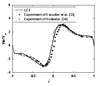
The dimensionless mean swirl velocity at the plane of Y/D = -2.7 using LES have been compared to the works of Escudier et al. [33] and Hoekstra [34] as depicted in Figure 2. The swirl velocity grows dramatically in the vortex core, then drops toward the wall. This is the result typically reported in literature as a radial transition between forced and free-vortex modes. The two modes are evidently shown in Figure 2 and compare well with the measured data. The overall agreement between the measurements and the predictions of this work are quite acceptable with an overall average deviation of less than 5%.
The dimensionless radial pressure or the pressure coefficient Cp is defined as
$C_{p}=\frac{2[p(\overline{r})-p(\overline{r}=1)]}{\rho V_{i n}^{2}} \quad, \overline{r}=\frac{r}{r_{o}}$ (25)
As shown in Figure 3, where r0 and Vin represent the radius of the separator and the mixture inlet velocity respectively, the predicted results of the radial pressure profile at the plane of Y/D= -2.7 were validated against the published work of Georgantas et al. [35]. The figure clearly shows that the LES model can capture the experimental data, and further indicates that, on the one hand, the supreme pressure happens at the wall of air separator, which is attributed to the effect of the two centrifugal forces, while, on the other, the minimum pressure occurs at the centerline.
In an attempt to explore the flow features of the separation process (mixture of air and water) that is taking place inside the double vortex separator, extensive simulated images that concern velocity field, pressure, and volume fraction will be shown and analyzed. Anatomy for separator behavior will include full simulated images using the LES. These images will explain the fields of axial, tangential and radial velocities, radial pressure distribution, and volume fraction features of the double-vortex air separator. In the present simulation the cross- sectional horizontal slices are selected at axial locations of Y/D = 0.13 (outlet-1), 0.067, 0.0, -0.2 (upper generator), -0.33, -0.67, -1.0, -1.33, -1.67 (outlet-2), -2.0, -2.33, -2.67, -3, -3.13 (lower generator), and -3.33 (bottom of separator).
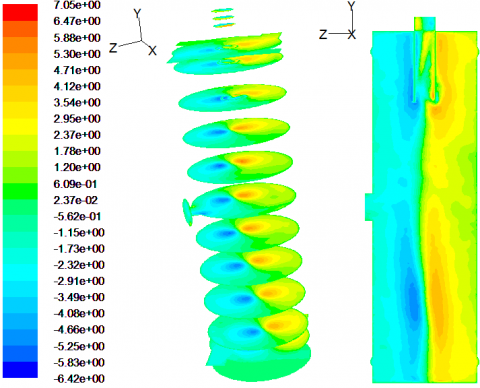
The present simulation captured the behavior of the axial velocity field inside the air separator as shown in Figure 4. The color contour plots of axial velocities clearly show the downward and upward flow regions that set a rotationary motion in the vertical plane. Typical flow patterns in the horizontal and vertical planes are depicted in Figs. 4(a) and 4(b). The latter figure indicates that LES can capture a phenomenon referred by several researchers including Erdal [21] and Hreiz et al. [20] as the vortex helical pitch.
Figure 2. Comparison of the dimensionless mean tangential (swirl) velocity at VF=95% and Re=8×10⁴
Figure 3. Comparison of the dimensionless radial pressure at VF = 95% and Re=8×10⁴
Figure 4. Contours of axial velocity (m/s) at VF=95% and Re=8×10⁴ (a) axial velocity field at different cross sectional horizontal slices, and (b) axial velocity filed along a vertical slice (Z=0).
The swirl velocity is the dominant velocity that has a direct influence on separation efficiency. Higher tangential velocity means higher centrifugal force that improves the separation efficiency. A typical tangential velocity field is depicted in Figure 5. Specifically, the contours of the tangential velocity field at different cross sectional horizontal slices, and along a vertical slice (X=0) are shown in Figs. 5(a) and 5(b), respectively. The tangential velocity is positive on one side and negative on the other. The forced and free vortex modes are captured where the core size structure has a wavy behaviour known as precessing vortex core (PVC) and this behaviour has been mentioned in literature such as (Darmofal et al. [36]; and Hoekstra [34]). Two generators, upper and lower, both of which work in clock-wise direction, are used to feed the separator. In order to get further details on the swirl velocity field, three axial locations, shown in Figure 6, were selected, namely, Y/D= -1.3, -2, and -2.7. Figure 6 shows that swirl velocity decays from the generator toward the mid of separator, which can be attributed to damping effects. The figure also shows that the vortex core expands toward the mid of separator resulting in lowering the vortex strength. Both of Figs 5(b) and 6 show that the location of the zero tangential velocity is off the center of the cylinder.
Figure 5. The contour of tangential velocity (m/s) at VF = 95% and Re=8×10⁴ (a) tangential velocity field at different cross sectional horizontal slices, and (b) tangential velocity field along a vertical slice (X=0).
Figure 6. Predicted swirl velocity at different axial locations.
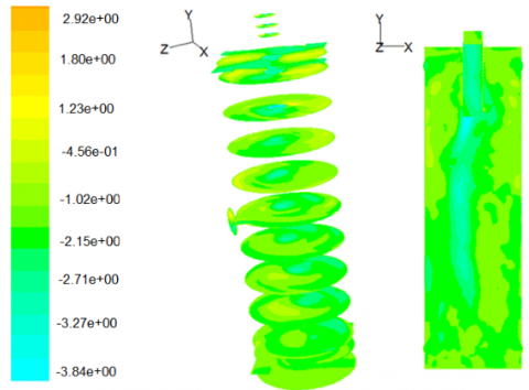
The radial velocity in literature has been considered as negligible except few researchers for instance Hreiz et al. [20] who referred that the radial velocity cannot be neglected in spite of its low value comparable to the swirl and axial velocities since all velocity are connected through the conservation of mass law. The present simulation confirms the previous conclusion that the radial velocity can’t be neglected as seen in Figure 7. The figure shows the contour of radial velocity at VF=95% and Re=8×10⁴ indicating that radial velocities are negative inside the vortex core where it exhibits different signs in free vortex region. And, to quantify the radial velocity field, three axial locations of Y/D = -2.7, -2, and -1.3, were selected as depicted in Figure 8. It may be noted that, in general, the values of radial velocity don’t exceed those of inlet velocity.
Figure 7. Contour of radial velocity(m/s) at VF=95% and Re=8×10⁴ (a) radial velocity field at different cross sectional horizontal slices, and (b) radial velocity field along a vertical slice (Z=0).
Figure 8. Predicted radial velocity at different axial locations
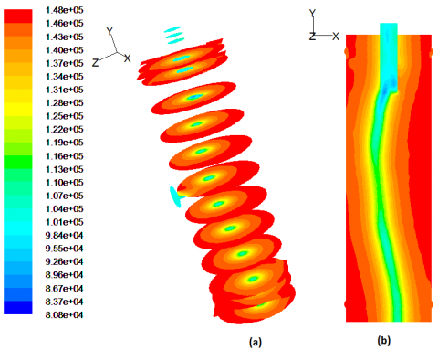
Figure 9. Contour of static pressure (pa) at VF=95% and Re=8x10⁴ (a) static pressure field at different cross sectional horizontal slices, and (b) static pressure field along a vertical slice (Z=0).
The contour of mixture static pressure field is given in Figure 9, where Figure 9(a) shows the mixture static pressure field at different cross sectional horizontal slices, and Figure 9(b) shows the mixture static pressure field along a vertical slice (Z=0). These figures clearly show that the pressure drops radially from the wall to the center of the air separator, which is in agreement with the swirl velocity behavior that changes from free to forced vortex mode as the flow approaches the axis of rotation. The pressure drops sharply reaching a value below the ambient pressure which causes reversal flow behavior of the axial velocity.
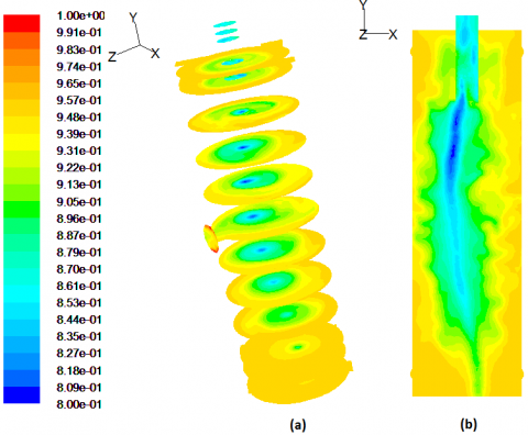
Simulated color contour plots of volume fraction are depicted in Figs. 10-12, which summarize the three cases of Table 2. The volume fraction fields at different cross sectional horizontal slices are depicted in Figs. 10-12(a), while volume fraction fields along a vertical slice (Z=0) are depicted given in Figs. 10-12(b). It is clear that phase-2 (air) is confined and localized along the centerline of the separator and then migrates toward the upper exit hole (outlet-1), while phase-1 (water) is expelled due to strong centrifugal forces and rotated along the wall and then directed to its exit hole (outlet-2).
In the process, two vortex generators impart momentum to the air-water mixture in clock-wise direction and then direct the mixture in the tangential direction along the separator. As the mixture starts rotating along the separator wall, a rotating liquid film with dispersed bubbles will form along the wall. Under the action of two strong centrifugal forces, the major bubbles tend to move in the radial direction toward the centerline and then the gas separates and adds to the inner gas stream in the axial direction toward upper exit hole (outlet-1). A large amount of air content in the mixture separates inside the core region where the pressure is too low. The separation process on the air-water mixture happens mainly due to the action of two strong centrifugal forces rather than the gravitational force, meaning that its footprint and weight are less than those in other conventional separators. The ideal operation of any separator is achieved when the inlet air-water mixture separates into two distinct clean streams, or if any phase content must be very small comparable to the other phase at the same outlet. Water carry-over, water content in the air stream, and gas carry-under, the air content in the water stream, are two important variables describe the efficiency of the air separator. Figs. 10-12 shows that the majority of water content is concentrated and separated at outlet-2 as seen from the red color, while the majority of air is concentrated and separated at outlet-1 as seen from the blue color.
Figure 10. Contour of volume fraction field at VF = 95% and Re=8×10⁴ (a) volume fraction field at different cross sectional horizontal slices, and (b) volume fraction field along a vertical slice (Z=0).
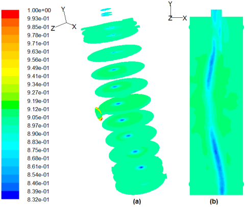
Figure 11. Contour of volume fraction field VF=90% and Re=8×10⁴ (a) volume fraction field at different cross sectional horizontal slices, and (b) volume fraction field along a vertical slice (Z=0).
Figure 12. Contour of volume fraction field VF = 95% and Re=2×10⁵ (a) volume fraction field at different cross sectional horizontal slices, and (b) volume fraction field along a vertical slice (Z=0).
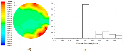
Figure 13. Volume fraction field at outlet-2 at VF=95% and Re=8×10⁴ (a) volume fraction contour, and (b) histogram of volume fraction
Histograms provide useful information regarding the separation efficiency, and a frequency distribution shows how often each phase occurs. Figure 13 shows the volume fraction contour and its histogram at outlet-2. The inlet mixture volume fraction is 95% with Reynolds number of 8x10⁴. It is easy to see that the water phase is heavily concentrated at the outlet-2 with a volume fraction ranging from 92 to 100% as shown in Figure 13. A 29.84% of the exit area has a volume fraction value exceeds 95% as depicted in Figure 13(b). Figure 14 shows the case of mixture volume fraction of 90% with Reynolds number of 8x10⁴. The water phase is also heavily concentrated at the outlet-2 with a volume fraction ranging from 90 to 100% as shown in Figure 14. A 42% of the exit area has a volume fraction value exceeds 90% as depicted in Figure 14(b). Figure 15 shows the case of mixture volume fraction of 95% with Reynolds number of 2x10⁵. Water volume fraction ranging from 95 to 100% as depicted in Figure 15. A 34.27% of the exit area has a volume fraction value exceeds 95% as depicted in Figure 15(b).
Figure 14. Volume fraction field at outlet-2 at VF=90% and Re=8×10⁴ (a) volume fraction contour, and (b) histogram of volume fraction.
Figure 15. Volume fraction field at outlet-2 at VF = 95% and Re=2×10⁵ (a) volume fraction contour, and (b) histogram of volume fraction.
In order to have a qualitative assesment of the separation performance, the average volume fraction is calculated via integration the annulus flow at outlet boundary in the numerical software, then the mass flowrate of separated water, ṁsw, and the inlet water, ṁiw, are calculated. Thereafter, the separation efficiency h is calculated according to the following equation:
$\eta=\frac{\dot{m}_{s w}}{\dot{m}_{n v}}$ (26)
For the case that appears in Figure 13(a), the separation efficiency through the outlet annulus with a hydraulic diameter of 16.7 mm or 66% of its area is 97.8%. For the next case that appears in Figure 14(a), the separation efficiency through the outlet annulus with a hydraulic diameter of 8.34 mm or 37.4% of its area is 96.1%. For the last case that appears in Figure 15(a), the separation efficiency through the outlet annulus with a hydraulic diameter of 18.4 mm or 70.8% of its area is 98.6%.
Practically, the water phase can be extracted from the annulus while at the core region the exiting mixture can be recirculated back to the vortex generators to refine the separation process again.
In order to compare the separator efficiency with other type of separators, Kurokawa and Ohtaik [37] have shown experimentally that the separation efficiency for a conventional separator is between 68% and 80%, and the separation efficiency for a single swirl generator is between 93% and 95% for different Reynolds numbers and feeding volume fractions, while the present study shows the separation efficiency using a double vortex generator is between 96.1% and 98.6%.
Air is a source of trouble in various applications such as liquid circulation in HVAC systems. Two vortex generators have been used to enhance the separation efficiency. The mixture multiphase and large eddy simulation (LES) turbulence models are capable to predict the mixture flow behaviour inside the air separator. The mixture multiphase and LES turbulence models were applied successfully. Current simulation showed the behavior of the axial velocity where the downward and upward flow regions, setting a rotationary motion in the vertical plane. The forced and free vortex modes for swirl velocity are captured where the core size structure has a wavy behaviour known as precessing vortex core. The radial velocity cannot be negligible in spite its low value comparable to the swirl and axial velocities. The static pressure decreases radially from the wall to the separator centre, the pressure drops sharply and its value reach below the ambient pressure which causes reversal flow behaviour of the axial velocity. Air phase was trapped and localized along the centerline of the separator and then migrated toward the upper exit hole, while water phase was distributed and rotated along the wall, then confined at the mid-separator as a result of two strong clock-wise centrifugal forces, and then expelled through its exit at mid of separator. It is revealed that the separation efficiency will increase as the Reynolds number increases and/or increasing the volume fraction.
|
A |
Area |
|
Cp |
Pressure coefficient |
|
D |
Diameter of the separator |
|
dp |
Diameter of the inclined hole |
|
F |
Body fore |
|
L |
Separator length |
|
M |
Mass flow rate |
|
P |
Static pressure |
|
R |
Radius |
|
$\overline{r}$ |
Normalized radius, r/ro |
|
Re |
Reynolds number |
|
ro |
Radius of the separator |
|
ui, uj, uk |
Velocity components in Cartesian coordinates |
|
Vj Vz,Vr |
Swirl, axial and radial velocity components |
|
V |
Velocity |
|
Vin |
Mixture inlet velocity |
|
VF |
Feeding Volume Fraction |
|
Greek Symbols |
|
|
e |
Turbulence dissipation rate |
|
m |
Dynamic viscosity |
|
K |
Turbulent kinetic energy |
|
r |
Density |
|
u |
Kinematics viscosity |
|
q |
Inlet angle |
|
h |
separation efficiency |
|
Subscripts |
|
|
a |
Air |
|
f |
Fluid |
|
in |
Inlet |
|
m |
Mixture |
|
r,j,z |
Radial, tangential and axial coordinate respectively |
|
t |
Turbulent |
[1] McQuiston P.J., Spitler J. (2005). Heating, Ventilating and Air Conditioning - Analysis & Design, 6th edition, F.C., Wiley and Sons, USA.
[2] Xia J.L., Yadigaroglu G. (1998). Numerical and experimental study of swirling flow in a model combustor, Int. J. Heat Mass Transfer, Vol. 41, No. 11, pp. 1485-1497.
[3] Smith, J.L. (1962). An experimental study of the vortex cyclone separator, J. Basic Engr., Vol. 84, pp. 602-608.
[4] Stairmand C.J. (1951). The design and performance of cyclone separators, Trans. IChem. E., Vol. 29, pp. 356-383.
[5] Hoffmann A.C., Van Santen A., Allen R.W.K. (1992). Effects of geometry and solid loading on performance of gas cyclones, Powder Technology, Vol. 70, pp. 83-91.
[6] Mondal S., Dattab A., Sarkar A. (2004). Influence of side wall expansion angle and swirl generator on flow pattern in a model combustor calculated with k-ε model, International Journal of Thermal Sciences, Vol. 43, pp. 901-914.
[7] Pisarev G.I., Hoffmann A.C. (2012). Effect of the ‘end of the vortex’ phenomenon on the particle motion and separation in a swirl tube separator, Powder Technology, Vol. 222, pp. 101-107
[8] Boivin M., Simonin O., Squires K.D. (2000). On the prediction of gas-solid flows with two-way coupling using large eddy simulation, Physics of Fluids, pp. 2080-2090.
[9] Bergstrom J., Vomhoff H. (2007). Review: Experimental hydrocyclone flow field studies, Separation and Purification Technology, Vol. 53, pp.8-20
[10] Erdal F.M., Shirazi S.A. (2004). Local velocity measurements and computational fluid dynamics (CFD) simulations of swirling flow in a cylindrical cyclone separator, Transactions of the ASME Journal of Energy Resources Technology, Vol. 126, pp. 326-3333.
[11] Hu L.Y., Zhou L.X., Zhang J., Shi M.X. (2005). Studies on strongly swirling flows in the full space of a volute cyclone separator, American Institute of Chemical Engineers, Vol. 51, pp. 740-749.
[12] Rosa E.S., Franc F.A., Ribeiro G.S. (2001). The cyclone gas-liquid separator: operation and mechanistic modeling, Journal of Petroleum Science and Engineering, Vol. 32, pp. 87-101.
[13] Bloor M.I.G, Ingham D.B. (1987). The flow in industrial cyclones, J Fluid Mech., Vol. 178, pp. 507-519.
[14] Hwang C.C, Shen H.Q, Zhu G, Khonsary M.M. (1983). On the main flow pattern in hydrocyclones, J. Fluids Eng, Vol. 115, pp. 21-25.
[15] Shi B., Wei J., Chen P. (2013). 3D turbulent flow modeling in the separation column of a circumfluent cyclone, Powder Technology, Vol. 235, pp. 82-90.
[16] Gao X., Chen J.F., Feng J.M., Peng X.Y. (2013). Numerical investigation of the effects of the central channel on the flow field in an oil-gas cyclone separator, Computers & Fluids, Vol. 20, pp. 45-55.
[17] Derksen J.J. (2005). Simulations of confined turbulent vortex flow, Computers & Fluids, Vol. 34, pp. 301-318.
[18] Shukla S.K., Shukla P., Ghosh P. (2013). The effect of modeling of velocity fluctuations on prediction of collection efficiency of cyclone separators, Applied Mathematical Modelling, Vol. 37, pp. 5774-5789.
[19] Elsayed K., Lacor C. (2013). The effect of cyclone vortex finder dimensions on the flow pattern and performance using LES, Computers & Fluids, Vol. 71, pp. 224-239.
[20] Hreiz R., Gentric C., Midoux N. (2011). Numerical investigation of swirling flow in cylindrical cyclones, Chemical Engineering Research and Design, Vol. 89, pp. 2521-2539.
[21] Erdal F. (2001). Local measurements and computational fluid dynamics simulations in a gas-liquid cylindrical cyclone separator, Ph.D. thesis, The University of Tulsa.
[22] Gupta A.K., Lilly D.G., Syred N.N. (1984). Swirl Flows, Abacus, Tunbridge Wells, England, UK.
[23] Jawarneh A.M., Vatistas G.H., Hong H. (2005). On the flow development in jet-driven vortex chambers, AIAA Journal of Propulsion and Power, Vol. 21, pp. 564-570.
[24] Yilmaz M., Çomakli Ö., Yapici S. (1999). Enhancement of heat transfer by turbulent decaying swirl flow, Energy Conversion and Management, Vol. 40, pp.1365-1376.
[25] Jawarneh A.M., Sakaris P., Vatistas G.H. (2007). Experimental and analytical study of the pressure drop across a double-outlet vortex chamber, Journal of Fluids Engineering, Vol. 129, No. 1, pp. 100-105.
[26] Jawarneh A.M. and Vatistas G.H. (2006). Reynolds stress model in the prediction of confined turbulent swirling flows, Journal of Fluids Engineering, Vol. 128, No. 6, pp. 1377-1382
[27] Jawarneh A.M., Al-Shyyab A, Tlilan H, Ababneh A. (2009). Enhancement of a cylindrical separator efficiency by using double vortex generators, Energy Conversion and Management, Vol. 50, No. 6, pp. 1625-1633.
[28] Jawarneh A.M., Tlilan H., Al-Shyyab A., Ababneh A. (2008). Strongly swirling flows in a cylindrical separator, Minerals Engineering, Vol. 21, No. 5, pp. 366-372.
[29] Fluent-UG, Fluent Inc. (2006). FLUENT 6.3 User’s Guide, Lebanon, NH.
[30] Hinze J.O. (1975). Turbulence, McGraw-Hill Publishing Co., New York.
[31] Smagorinsky J. (1963). General circulation experiments with the primitive equations. I. The basic experiment, Month. Wea. Rev., pp. 91, 99-164.
[32] Patankar S.V. (1980). Numerical Heat Transfer and Fluid Flow, Hemisphere, Washington D.C.
[33] Escudier M.P., Bornstein J., Zehnder N. (1980). Observations and LDA measurements of confined turbulent vortex flow, J Fluid Mech, Vol. 98, pp. 49-63.
[34] Hoekstra A.J. (2000). Gas flow and collection efficiency of cyclone separators, Ph.D. Thesis, Delft University of Technology.
[35] Georgantas A.I., krepec T., Kwork C.K. (1986). Vortex flow patterns in a cylindrical chamber, AIAA/ASME fouth fluid mechanics, plasma dynamics and laser conference, AIAA-86-1098, Atlanta, GA, May 12-14.
[36] Darmofal D.L., Khan R., Greitzer E.M., Tan C.S. (2001). Vortex core behaviour in confined and unconfined geometries: a quasi-one-dimensional model, J. Fluid Mech., Vol. 449, pp. 61-84.
[37] Kurokawa J., Ohtaik T. (1995). Gas-liquid flow characteristics and gas-separation efficiency in a cyclone separator, ASME FED, Vol. 225, pp. 51-57.