OPEN ACCESS
Entropy generation and irreversibility distribution due to steady mixed convection flow of a viscous incompressible fluid between two vertical parallel porous plates is investigated in the present study. The mathematical model capturing this physical situation was formulated considering internal heat generation and viscous dissipation within the channel. Combining the viscous dissipation effect with mixed convection lead to nonlinearity of the energy equation as well as coupling of the energy with the momentum equations. Due to the coupling and nonlinearity associated with the energy and momentum equations, obtaining a closed form solution becomes practically infeasible; therefore approximate solutions to the governing equations are obtained using the Homotopy Perturbation Method (HPM). The impacts of the several governing parameters on the velocity, temperature, the entropy generation number including the irreversibility distribution ratio were investigated and discussed. From the course of investigation, it was revealed that entropy generation number decreases near the centre line of the channel and higher near the porous plates. It is also discovered that fluid friction irreversibility dominates entropy generation towards the channels porous walls while heat transfer irreversibility dominates towards the centerline of the channel.
entropy generation, mixed convection, homotopy perturbation, irreversibility distribution
Irreversible processes can cause entropy of a system to change. The second law of thermodynamics accounts for irreversibility or entropy. Sources of irreversibility include; heat transfer across finite temperature difference, unrestrained chemical reaction, fluid viscosity, turbulence, and so on. Entropy change due to irreversibility is called entropy generation and this is encountered in all thermal systems. One of the significant interests in thermal systems is to minimize energy losses and fully maximize the energy resources. Investigation of mixed convection flow in a vertical porous channel is of special importance in view of its numerous applications in engineering and industries such as petroleum reservoirs, geothermal reservoirs, nuclear reactor cooling, thermal insulation, metallurgy, energy storage and conservation as well as chemical and food industries. The study of entropy generation in porous channel has attracted the attention of researchers in recent times. Bejan [1-3] pioneered theoretical work on entropy generation in flow systems. He showed that efficiency of a machine can be improved by minimizing entropy generation. Makinde and Eegunjobi [4] utilized velocity and temperature profiles to compute entropy generation in a couple stress fluid flows through a vertical channel. They affirmed that velocity profiles are parabolic in nature. Other several authors [5-13] have investigated different problems to analyze effects of entropy on thermal systems and to proffer ways to minimize them.
Ajibade et al. [14] investigated entropy generation under the effect of suction. In the work of Ajibade et al. [14] entropy generation and irreversibility distribution were obtained and analyzed for a pressure driven flow through a porous horizontal channel. The set-up of the problem shows that the energy in the system is due to asymmetric heating of the porous channel plates and the viscous dissipation within the channel. It is however observed that despite the temperature gradient generated by the thermal input into the system, the buoyancy effect on the fluid was completely ignored. This is due to the channel orientation which is in the horizontal position.
When the channel orientation is changed from horizontal through certain inclinations to vertical, the influence of acceleration due to gravity comes into play. In this case, the mass flux is influenced by the applied temperature and the problem becomes a mixed convection flow. It is therefore necessary to introduce a new parameter called the mixed convection parameter which is used to regulate the relative contributions of forced convection and that of natural convection within the system.
Mahmud and Fraser [15] studied Entropy generation in mixed convection-radiation interaction in a vertical porous channel. Avci and Aydin [16] investigated mixed convection flow in a vertical microchannel considering asymmetric but isothermal heating of the channel plates. In a related work, Avci and Aydin [17] investigated a similar problem in which the energy within the system is due to asymmetric heat fluxes on the boundaries. Barletta and Zanchini [18] and Zanchini [19] are two other works that investigated mixed convection flow; the former investigated the problem in a vertical channel while the latter was investigated in a vertical annulus subjected to uniform wall temperature. Avci and Aydin [20] investigated mixed convection in a vertical microannulus and concluded that increasing the mixed convection parameter enhances heat transfer while rarefaction decreases it. Jha et al. [21] investigated steady mixed convection in a microchannel filled with porous material. They found that growing the porosity of the medium decreases the critical value of the mixed convection parameter which signaled the onset of reverse flow in the channel. In another article, Jha et al. [22] investigated the role of porous medium in a mixed convection flow in a vertical tube with time periodic boundary condition. The work identifies a stagnation point within the tube and confirms that variations in fluid type, porosity as well as frequency have no impact on fluid velocity at this section. Seth et al. [23] investigated unsteady hydromagnetic convective flow of a viscous incompressible electrically conducting heat generating/absorbing fluid within a parallel plate rotating channel in a uniform porous medium under slip boundary conditions. Among their findings is that thermal source tends to accelerate fluid flow in both the primary and secondary flow directions whereas thermal sink has reverse effect on it. Seth et al.[24] studied the effects of Hall current on unsteady hydromagnetic free convection flow with heat and mass transfer of an electrically conducting, viscous, incompressible and time dependent heat absorbing fluid past an impulsively moving vertical plate in a porous medium, in the presence of thermal diffusion. They indicated that heat absorption enhances rate of heat transfer at the plate whereas thermal diffusion has a reverse effect on it, and as time progresses, rate of heat transfer at ramped temperature plate is getting enhanced whereas it is getting reduced for isothermal plate. In a related article, Seth et al. [25] concluded that heat absorption has tendency to reduce fluid temperature whereas fluid temperature is getting enhanced with the progress of time. Also, Seth et al. [26] investigated unsteady MHD natural convection flow with Hall effects of an electrically conducting, viscous, incompressible and heat absorbing fluid past an exponentially accelerated vertical plate with ramped temperature through a porous medium in the presence of thermal diffusion. They observed that heat absorption tends to decelerate fluid flow in both the primary and secondary flow directions as well as enhance rate of heat transfer at the plate and that rate of heat transfer at the plate increases with time. In Seth et al. [27] it was observed that heat absorption tended to enhance rate of heat transfer at the moving plate whereas it had a reverse effect on the rate of heat transfer at the stationary plate.
In this paper, we extend the work of Ajibade et al. [14] to investigate entropy generation due to a mixed convection flow through a vertical porous channel. The temperature and velocity field are obtained and discussed for some carefully selected values of the flow parameters.
The present problem considers steady mixed convection flow of viscous incompressible fluid in a vertical channel formed by two infinite parallel porous plates. The $x^{\prime}$ axis is taken vertically parallel to one of the porous plates of the channel and normal to the $y^{\prime}$ axis. The porous plates are stationary and parallel to each other at distance 2$l$ apart as shown in Figure 1. The fluid flow is set up due to the applied pressure gradient along channel walls as well as density change caused by the asymmetric heating of the channel boundary porous plates and under the action of gravitational force, hence, the present situation describes a mixed convection flow in a vertical porous channel.
Figure 1. Schematic diagram of the flow
In addition, heat transfer in the system is due to the isothermal heating of one of the porous plates as well as viscous dissipation within the channel and under the action of heat generation/absorption. Also, we assume the flow to be steady and fully developed; hence, the temperature and velocity fields are functions of $y^{\prime}$ alone.
The governing equations for the steady flow of viscous incompressible fluid between two heated parallel plates are the conservation of mass
$\nabla \vec{V}=0$ (1)
conservation of momentum
$(\vec{V} . \nabla) \vec{V}=v \nabla^{2} \vec{V}-\frac{1}{\rho} \nabla P+g \beta\left(T^{\prime}-T_{0}\right)$ (2)
and the conservation of energy
$(\vec{V} . \nabla) T=\frac{k}{\rho C_{P}} \nabla^{2} T+\frac{\mu}{\rho C_{P}}(\nabla u)^{2}+\frac{Q_{0}\left(T^{\prime}-T_{0}\right)}{\rho C_{P}}$ (3)
where $\nabla=\frac{\partial}{\partial x} i+\frac{\partial}{\partial y} \underline{j}+\frac{\partial}{\partial z} \underline{k}$ . The physical quantities, $\rho$ ,$\vec{V}$ , $\mathbf{v}$ , $k$ and P are defined in the nomenclature.
Considering a two dimensional velocity so that $\vec{V}=\left(u^{\prime}, v^{\prime}, 0\right)$ , where $\mathcal{u}^{\prime}$and $\boldsymbol{v}^{\prime}$ are the vertical and horizontal (suction/injection) components of the velocity respectively. Since the flow is assumed to be fully developed, the conservation of mass equation (1) is reduced to
$\frac{d v^{\prime}}{d y^{\prime}}=0$ (4)
Upon integration of eq. (4), we obtain the horizontal velocity as a constant (say, $v^{\prime}=-v_{0}$ ) which is the velocity of suction/injection.
The equations of motion for steady mixed convection flow of a viscous incompressible heat generating fluid with viscous dissipation are given as,
$v \frac{d^{2} u^{\prime}}{d y^{2}}+v_{0} \frac{d u^{\prime}}{d y^{\prime}}-\frac{1}{\rho} \frac{\partial P}{\partial x^{\prime}}+g \beta\left(T^{\prime}-T_{0}\right)=0$ (5)
$\frac{k}{\rho C_{p}} \frac{d^{2} T^{\prime}}{d y^{2}}+v_{0} \frac{d T^{\prime}}{d y^{\prime}}+\frac{\mu}{\rho C_{P}}\left(\frac{d u^{\prime}}{d y^{\prime}}\right)^{2}+\frac{Q_{0}\left(T^{\prime}-T_{0}\right)}{\rho C_{P}}=0$ (6)
while the boundary conditions are
$u^{\prime}=0, T^{\prime}=T_{0}$ at $y^{\prime}=-l$
$u^{\prime}=0, T^{\prime}=T_{w}$ at $y^{\prime}=l$$\}$ (7)
The following non-dimensional quantities are used to transform equations (5) – (7) to dimensionless form.
$y=\frac{y^{\prime}}{l}, \theta=\frac{T^{\prime}-T_{0}}{T_{w}-T_{0}}, S=\frac{v_{0} l}{v}, \operatorname{Pr}=\frac{\mu C_{P}}{k}, E c=\frac{U^{2}}{C_{P}\left(T_{w}-T_{0}\right)}$
$u=\frac{u^{\prime}}{u_{0}^{\prime}}, \quad G r=\frac{g \beta l^{3}\left(T_{w}-T_{0}\right)}{v^{2}}, \operatorname{Re}=\frac{l u_{0}}{v}, \delta=\frac{Q_{0} l^{2}}{k}$$\}$ (8)
Substituting equation (8) into equations (5) and (6), the momentum and energy equations are rendered in dimensionless form as
$\frac{d^{2} u}{d y^{2}}+S \frac{d u}{d y}-\gamma+\frac{G r}{\operatorname{Re}} \theta=0$ (9)
$\frac{d^{2} \theta}{d y^{2}}+S \operatorname{Pr} \frac{d \theta}{d y}+E c \operatorname{Pr}\left(\frac{d u}{d y}\right)^{2}+\delta \theta=0$ (10)
and the boundary conditions are given as
$u=0, \theta=0$ at $y=-1$
$u=0, \theta=1$ at $y=1$$\}$ (11)
where $\gamma=\frac{l^{2}}{\mu u_{0}} \frac{\partial P}{\partial x^{\prime}}$
For brevity, we shall write the mixed convection parameter $G r / \mathrm{Re}$ as Gre . This parameter measures the contribution of either the forced convection (small value of Gre) or natural convection (large value of Gre ). For mixed convection, a moderate value of Gre is required. $P r$ is the Prandtl number which is inversely proportional to the thermal diffusivity of the fluid. S is the dimensionless suction/injection parameter, where positive values denote suction at the porous plate $\left(y^{\prime}=-l\right)$ with a corresponding injection on the plate $y^{\prime}=l$ while negative values denote injection at the porous plate $y^{\prime}=-l$ with a corresponding suction on the other plate. Eckert number ( $E c$ ) is the measure of viscous dissipation in the system while $\delta$ is the temperature dependent heat source/sink parameter, positive values of $\delta$ represent heat source and negative values represent heat sink. All the physical quantities used in the dimensionless analysis are defined in the nomenclature.
In order to solve equations (9) and (10) subject to the boundary conditions (11), we use the Homotopy perturbation method (HPM) to obtain approximate analytical solutions to the problem. HPM is a powerful solution tool to solve linear as well as nonlinear equations. The method has been shown to perform excellently well in solving this type of problems [28] and is advantageous over the regular perturbation technique because it was able to overcome the small parameter restriction which characterizes the regular perturbation technique.
2.1 Homotopy perturbation method
In order to illustrate the basic ideas of the HPM, we consider the following nonlinear differential equation
$A(u)-f(r)=0, r \in \Omega$ (12)
$B\left(u, \frac{\partial u}{\partial r}\right)=0, r \in \Gamma$ (13)
where $A$ is a general differential operator, $B$ is a boundary operator, $f(r)$ is a known analytic function, $\Gamma$ is the boundary of the domain $\Omega$ . The operator $A$ can be divided into two parts $L$ and $N$ , where $L$ is linear and $N$ is nonlinear. Hence, eq. (12) can be rewritten as
$L(u)+N(u)-f(r)=0$ (14)
Using the Homotopy perturbation technique, we construct a Homotopy $v(r, P) : \Omega \times[0,1] \rightarrow R$ which satisfies
$H(v, P)=(1-P)\left[L(v)-L\left(u_{0}\right)\right]+P[A(v)-f(r)]=0, P \in[0,1], r \in \Omega$ (15)
or
$\mathrm{H} \quad(v, P)=L(v)-L\left(u_{0}\right)+P L\left(u_{0}\right)+P[N(u)-f(r)]=0$ (16)
where $P \in[0,1]$ is called the Homotopy parameter, $u_{0}$ is the initial approximation for the solution of eq. (12) which satisfies the boundary conditions. Clearly, from eqs. (15) and (16) we have;
$\mathrm{H} \quad(v, 0)=L(v)-L\left(u_{0}\right)=0$ (17)
$\mathrm{H} \quad(v, 1)=A(v)-f(r)=0$ (18)
Assuming that the solution of eqs. (15) and (16) are expressed as a power series in $P$ , that is
$v=v_{0}+P v_{1}+P^{2} v_{2}+\ldots$ (19)
Setting $P=1$ gives the approximate solution of eq. (12) as
$u=\lim _{P \rightarrow 1} v=v_{0}+v_{1}+v_{2}+\cdots$ (20)
Applying the Homotopy perturbation technique to solve the governing equations in the present problem, we construct Homotopy on eqs. (9) and (10) to get
$H(u, P)=(1-P)\left(\frac{d^{2} u}{d y^{2}}+G r e \theta\right)+P\left(\frac{d^{2} u}{d y^{2}}+S \frac{d u}{d y}+G r e \theta-\gamma\right)=0$ (21)
$H(\theta, P)=(1-P)\left(\frac{d^{2} \theta}{d y^{2}}\right)+P\left(\frac{d^{2} \theta}{d y^{2}}+S \operatorname{Pr} \frac{d \theta}{d y}+E c \operatorname{Pr}\left(\frac{d u}{d y}\right)^{2}+\delta \theta\right)=0$ (22)
Simplifying
$\frac{d^{2} u}{d y^{2}}+G r e \theta+P\left(S \frac{d u}{d y}-\gamma\right)=0$ (23)
$\frac{d^{2} \theta}{d y^{2}}+P\left(S \operatorname{Pr} \frac{d \theta}{d y}+E c \operatorname{Pr}\left(\frac{d u}{d y}\right)^{2}+\delta \theta\right)=0$ (24)
Assume the solutions of eqs. (9) and (10) to be written as
$u=u_{0}+P u_{1}+P^{2} u_{2}+\ldots$
$\theta=\theta_{0}+P \theta_{1}+P^{2} \theta_{2}+\ldots$$\}$ (25)
Substituting eq. (25) into eqs. (23) and (24) and simplifying, we have the following sets of boundary value problems which are obtained by comparing the coefficients of powers of $P$ .
Zeroth order:
$\frac{d^{2} \theta_{0}}{d y^{2}}=0$ (26)
$\frac{d^{2} u_{0}}{d y^{2}}+G r \theta_{0}=0$ (27)
$\begin{array}{ll}{\theta_{0}(-1)=0,} & {u_{0}(-1)=0} \\ {\theta_{0}(1)=1,} & {u_{0}(1)=0}\end{array}$ (28)
First order:
$\frac{d^{2} \theta_{1}}{d y^{2}}+S \operatorname{Pr} \frac{d \theta_{0}}{d y}+E c \operatorname{Pr}\left(\frac{d u_{0}}{d y}\right)^{2}+\delta \theta_{0}=0$ (29)
$\frac{d^{2} u_{1}}{d y^{2}}+G r e \theta_{1}+S \frac{d u_{0}}{d y}-\gamma=0$ (30)
$\begin{array}{ll}{\theta_{1}(-1)=0,} & {u_{1}(-1)=0} \\ {\theta_{1}(1)=0,} & {u_{1}(1)=0}\end{array}$ (31)
Second order:
$\frac{d^{2} \theta_{2}}{d y^{2}}+S \operatorname{Pr} \frac{d \theta_{1}}{d y}+2 E c \operatorname{Pr}\left(\frac{d u_{0}}{d y}\right)\left(\frac{d u_{1}}{d y}\right)+\delta \theta_{1}=0$ (32)
$\frac{d^{2} u_{2}}{d y^{2}}+G r e \theta_{2}+S \frac{d u_{1}}{d y}=0$ (33)
$\begin{array}{ll}{\theta_{2}(-1)=0,} & {u_{2}(-1)=0} \\ {\theta_{2}(1)=0,} & {u_{2}(1)=0}\end{array}$ (34)
Solving the sets of Boundary Value Problems and taking limit as $P \rightarrow 1$ , the solution of the momentum and energy equations are
$u(y)=u_{0}(y)+u_{1}(y)+u_{2}(y) \cdots$ (35)
$\theta(y)=\theta_{0}(y)+\theta_{1}(y)+\theta_{2}(y)+\cdots$ (36)
where:
$u_{0}(y)=a_{1} y^{3}+a_{2} y^{2}+c_{3} y+c_{4}$
$u_{1}(y)=b_{1} y^{8}+b_{2} y^{7}+b_{3} y^{6}+b_{4} y^{5}+b_{5} y^{4}+b_{6} y^{3}+b_{7} y^{2}+c_{7} y+c_{8}$
$u_{2}(y)=g_{1} y^{3}+g_{2} y^{12}+g_{3} y^{11}+g_{4} y^{10}+g_{5} y^{9}+g_{6} y^{8}+g_{7} y^{7}+g_{8} y^{6}+g_{9} y^{5}+$ $g_{10} y^{4}+g_{11} y^{3}+g_{12} y^{2}+c_{11} y+c_{12}$
$\theta_{0}(y)=\frac{1}{2} y+\frac{1}{2}$
$\theta_{1}(y)=a_{3} y^{6}+a_{4} y^{5}+a_{5} y^{4}+a_{6} y^{3}+a_{7} y^{2}+c_{5} y+c_{6}$
$\theta_{2}(y)=d_{1} y^{11}+d_{2} y^{10}+d_{3} y^{9}+d_{4} y^{8}+d_{5} y^{7}+d_{6} y^{6}+d_{7} y^{5}+d_{8} y^{4}+d_{9} y^{3}+d_{10} y^{2}+c_{9} y+c_{10}$
The constants $a_{i}(i=1,2, \cdots 7)$ , $b_{i}(i=1,2, \cdots 7)$ , $c_{i}(i=1,2, \cdots 12)$ $d_{i}(i=1,2, \cdots 10)$ and $g_{i}(i=1,2, \cdots 12)$ are defined in the appendix.
2.2 Entropy generation in the system
For the flow of a Newtonian incompressible fluid due to Fourier law of heat conduction, the volumetric rate of entropy generation rate is given by Bejan2 in Cartesian coordinates as
$E_{G}=\frac{k}{T_{0}^{2}}\left(\left(\frac{\partial T}{\partial x}\right)^{2}+\left(\frac{\partial T}{\partial y}\right)^{2}\right)+\frac{\mu}{T_{0}}\left(2\left\{\left(\frac{\partial u}{\partial x}\right)^{2}+\left(\frac{\partial v}{\partial y}\right)^{2}\right\}+\left[\frac{\partial u}{\partial y}+\frac{\partial v}{\partial x}\right]^{2}\right)$ (37)
This form of entropy generation shows that the irreversibility results from two effects; conductive $(k)$ and viscosity $(\mu)$ . Entropy generation rate is finite and positive whenever one of temperature or velocity gradients is present in a medium. Velocity and temperature distribution are often simplified in many fundamental convective heat transfer problems, assuming that the flow is hydro-dynamically developed $\left(\frac{\partial \vec{V}}{\partial x}=0\right)$ and thermally developing $\left(\frac{\partial T}{\partial x} \neq 0\right)$ or thermally developed $\left(\frac{\partial T}{\partial x}=0\right)$ ( White [29] and Burmeister [30]), then eq. (37) is reduced to the form:
$E_{G}=\frac{k}{T_{0}^{2}}\left(\left(\frac{\partial T}{\partial x}\right)^{2}+\left(\frac{\partial T}{\partial y}\right)^{2}\right)+\frac{\mu}{T_{0}}\left(\frac{\partial u}{\partial y}\right)^{2}$ (38)
By scaling the velocity $u$ with the reference velocity $u_{0}$ , the distance $y$ with $l$, the distance $x$ with $l^{2} u_{0} \alpha^{-1}$ and expressing the dimensionless temperature $\theta$ as $\left(T-T_{0}\right) \Delta T^{-1}$ , the entropy generation is rendered in dimensionless form as
$N_{S}=\frac{1}{P e^{2}}\left(\frac{\partial \theta}{\partial x}\right)^{2}+\left(\frac{\partial \theta}{\partial y}\right)^{2}+\frac{B r}{\Omega}\left(\frac{\partial u}{\partial y}\right)^{2}=N_{c}+N_{y}+N_{f}$ (39)
where $P e=l u_{0} \alpha^{-1}$ is the Peclet number, and $\Omega=\Delta T / T_{0}$ is the dimensionless temperature difference. The first term $\left(N_{c}\right)$ stands for the entropy generation by heat transfer due to axial conduction, the middle term $\left(N_{y}\right)$ represents entropy generation due to heat transfer across different fluid sections within the channel, and the last term $\left(N_{f}\right)$ gives the contribution of viscous dissipation to entropy generation.
Substituting eqs. (35) and (36) into the dimensionless expression for entropy as presented in eq. (39), we have
$N_{s}=\lambda_{3}^{2}+B r \Omega^{-1} \lambda_{4}^{2}$ (40)
where:
$\frac{d \theta}{d y}=\lambda_{3}=11 d_{1} y^{10}+10 d_{2} y^{9}+9 d_{3} y^{8}+8 d_{4} y^{7}+7 d_{5} y^{6}+\left(6 a_{3}+6 d_{6}\right) y^{5}$ $+\left(5 a_{4}+5 d_{7}\right) y^{4}+\left(4 a_{5}+4 d_{8}\right) y^{3}+\left(3 a_{6}+3 d_{9}\right) y^{2}+\left(2 a_{7}+2 d_{10}\right) y+\left(\frac{1}{2}+c_{5}+c_{9}\right)$
$\frac{d u}{d y}=\lambda_{4}=13 g_{1} y^{12}+12 g_{2} y^{11}+11 g_{3} y^{10}+10 g_{4} y^{9}+9 g_{5} y^{8}+\left(8 b_{1}+8 g_{6}\right) y^{7}$ $+\left(7 b_{2}+7 g_{7}\right) y^{6}+\left(6 b_{3}+6 g_{8}\right) y^{5}+\left(5 b_{4}+5 g_{9}\right) y^{4}+\left(4 b_{5}+4 g_{10}\right) y^{3}$ $+\left(3 a_{1}+3 b_{6}+3 g_{11}\right) y^{2}+\left(2 a_{2}+2 b_{7}+2 g_{12}\right) y+\left(c_{3}+c_{7}+c_{11}\right)$
2.3 Irreversibility distribution ratio
Entropy generation rate is accounted for by both heat transfer and fluid friction in a convective problem. Eq. (39) shows the level of distribution of entropy but is unable to point out the relative contributions of each irreversibility to the total entropy generation. To identify whether it is the fluid friction or heat transfer irreversibility that dominates the total entropy, Bejan [1] defined irreversibility distribution ratio $\varphi$ as the ratio of the entropy generation due to fluid friction $\left(N_{f}\right)$ to heat transfer $\left(N_{c}+N_{y}\right)$ . However, Paoletti et al. [31]
showed an alternative irreversibility distribution parameter in terms of the Bejan number (Be) and defined it as the ratio of the entropy generation due to heat transfer $\left(N_{c}+N_{y}\right)$ to the entropy generation $\left(N_{s}\right)$ In the present problem, the flow is assumed to be thermally developed so that heat transfer due to axial conduction becomes negligible so that Bejan number becomes
$B e=\frac{N_{y}}{N_{s}}$ (41)
A critical look at the Bejan number shows that $0 \leq B e \leq 1$ with $B e=1$ indicating that the entropy generation is only by heat transfer irreversibility, whereas, $B e=0$ signify that the total entropy generation is as a result of fluid friction irreversibility only, whenever heat transfer and fluid friction contribute equally to the total entropy generation then $B e=1 / 2$ . In the light of this analysis, heat transfer irreversibility dominates the total entropy generation whenever $B e \rightarrow 1$ and likewise fluid friction irreversibility dominates when $B e \rightarrow 0$
$B e=\frac{\lambda_{3}^{2}}{\lambda_{3}^{2}+B r \Omega^{-1} \lambda_{4}^{2}}$ (42)
2.4 Pressure gradient
In order to estimate the pressure gradient in the present problem, we assumed that the flow has a constant mass flux so that $\gamma$ is obtained such that the mass flux within the channel is maintained at a constant level. That is
$\int_{-1}^{1} u(y) d y=2$ (43)
Upon evaluation of eq. (43), we have the following polynomial equation
$n_{4} \gamma^{3}+n_{8} \gamma^{2}+n_{9} \gamma+n_{10}=0$ (44)
where the expressions for $n_{i,} \quad i=0,1, \cdots 11$ are defined in the appendix.
The roots of the cubic equation (44) are obtained numerically using an in-built function on the platform of MATLAB.
2.5 Validation of results
By setting the heat generation term $\delta$ and the mixed convection term Gre to zero in the present problem, we recover the results of Ajibade et al. [14] The comparison is presented in the table below
Table 1. Numerical comparison between the present problem and case 2 of Ajibade et al. [14]
|
|
Ajibade et al. [14] $y=0$ |
Present problem Setting $G r e=0$ , $\delta=0$ , $y=0$ |
||
|
$S$ |
$\theta$ |
$u$ |
$\theta$ |
$u$ |
|
-1.0 |
0.344861366004390 |
0.462117157260010 |
0.344914877500000 |
0.458333333333333 |
|
-0.5 |
0.429243102325639 |
0.489837324807418 |
0.429234159479167 |
0.489583333333333 |
|
0.5 |
0.604902179290661 |
0.489837324807418 |
0.604870039687500 |
0.489583333333333 |
A slight deviation is observed in the values displayed in the table and this could be attributed to the different pressure gradients used in both problems. For instance, in the work of Ajibade et al. [14], the pressure gradient was assumed to be constant. However, the pressure gradient in the present problem is obtained from the evaluation of the constant mass flux equation (43). This means that the pressure gradient in the present problem is dependent on all other parameters that affect the velocity of the fluid.
This problem considers a mixed convection flow between two vertical porous plates with temperature-dependent heat generation and viscous dissipation. The non-dimensional parameters governing the fluid flow are; the mixed convection parameter ( Gre ), heat source/sink parameter $\delta$ , Prandtl number (Pr), suction/injection parameter (S) and the Eckert number $E_{C}$ . In this discussion, the value of Pr used is 0.71 which corresponds to the Prandtl number of air at 2.0 atm., S is chosen from -1.5 to 2.0 to account for injection as well as suction through the porous plates. The values of $\delta$ are chosen between -2.2 and 2.2 to accommodate both heat source $(\delta>0)$ and heat sink $(\delta<0)$ . Similarly, the value of Gre is selected arbitrarily between 5 and 25.
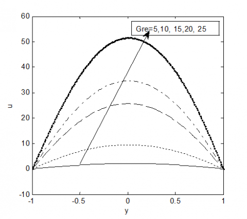
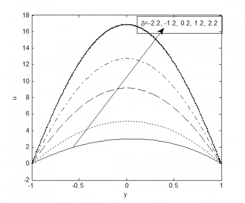
The influences of the governing parameters on the velocity are shown in figures 2 and 3. It can be seen that velocity increases with growing Gre and $\delta$ respectively. Physically speaking, higher value of Gre implies an enhanced buoyancy force which is higher when compared to the viscous force. This acts to thicken the momentum boundary layer hence, the fluid velocity increases with growing Gre. Similarly, velocity increase due to increase in heat generation $(\delta>0)$ could be hinged on heat accumulation within the channel which lead to a decrease in the density of the fluid resulting in enhanced buoyancy and hence, velocity increase. On the other hand, velocity decreases with increase in heat absorption $(\delta<0)$. This is physically true because heat sink acts to decrease the fluid temperature and this thins the thermal boundary layer hence, heat is being conducted away from the system leading to a rise in density of the fluid thereby decreasing the flow velocity.
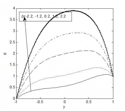
Figures 4 and 5 present temperature distribution within the channel for different values of Gre and $\delta$ . It could be viewed from figure 4 that growing Gre leads to a corresponding rise in temperature. This could be attributed to increase in buoyancy force against viscous force which characterizes growing Gre . It is also observed that there is an increase in temperature with increase in heat source $(\delta>0)$ which means that heat generation within the system exceeds conduction and this leads to heat accumulation. On the other hand, increasing heat sink $(\delta<0)$ implies higher conduction in excess of heat generation, leading to a decrease in the temperature within the channel.
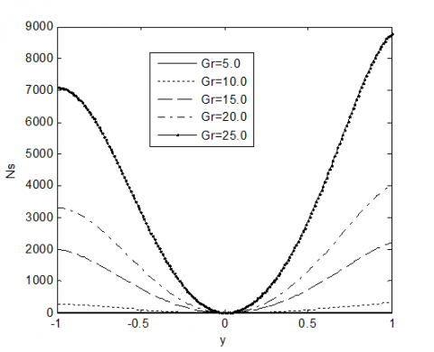
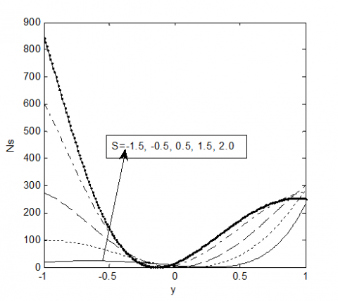
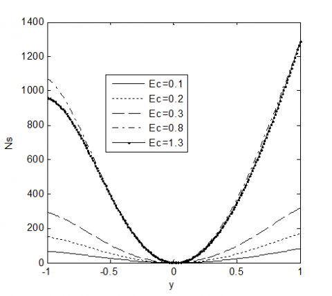
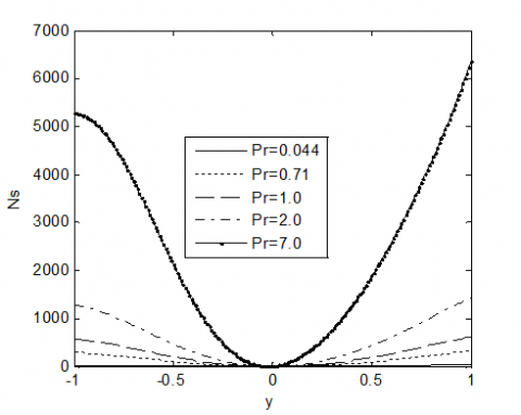
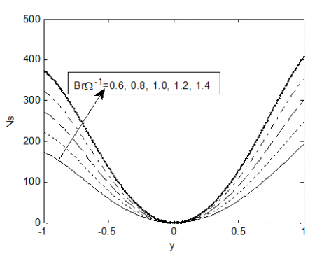
Figures 6-11 show effects of the operating parameters on the entropy generation number within the channel. It can be clearly viewed that minimum entropy generation is obtained at the centerline of the channel. However, entropy generation number increases with growing values of each of the parameters towards the porous walls. Maximum entropy generation number is obtained at the porous walls as revealed in figures 6-11. From Figure 6, it is observed that entropy generation increases near both porous plates with growing buoyancy. This is premised on the fact that increasing Gre leads to growing velocity and temperature which in turn increase the velocity and temperature gradients near the porous plates. However, the entropy generation decreases center wards and is minimal near the centerline; this is because velocity gradient is higher near the porous plates and decreases to zero as the centerline is approached from both plates. Also, it is observed in Figure 7 that increase in heat generation lead to growing entropy while increase in heat absorption acts to decrease the total entropy within the system.
The effect of channel porosity on entropy generation number as shown in Figure 8 reveals that increase in suction through the plate $y=1$ $(S>0)$ causes an increase in entropy generation near this plate. It is further revealed that injection through the plate $y=-1$ $(S<0)$ acts to decrease the entropy generation. Response of the entropy generation due to variations in the viscous dissipation parameter $(E c)$ is shown in Figure 9. The figure shows that entropy generation increases as the viscous dissipation is enhanced with growing $E c$ . A similar trend is observed in figure 10 in which entropy generation increases with growing Pr . This is physically true since growing $\mathrm{Pr}$ decreases thermal diffusivity of the fluid, therefore the diffusion of heat generated by viscous dissipation decreases as Pr increases, causing heat accumulation, hence increase in velocity as well as increase in entropy generation. A careful scrutiny of figs. 7-10 reveals that all parameters that cause temperature increase also causes entropy increase within the channel. From figure 11, entropy generation is observed to increase with increase in the group parameter $\left(B r \Omega^{-1}\right)$ . This is because growing the group parameter increases the contribution of fluid friction irreversibility to the total entropy generation.
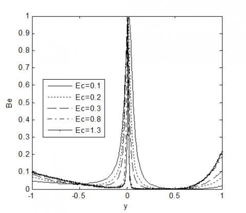
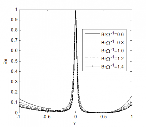
Figures 12-17 reveal the influence of the different flow parameters on the relative contribution of either the fluid friction irreversibility or heat transfer irreversibility to the total entropy generation within the channel. It is observed that fluid friction irreversibility dominates the total entropy generation towards the channel porous walls while heat transfer irreversibility dominates at the centerline of the channel. From Figure 12, it is observed that increase in Gre , which increases fluid velocity has consequently lead to an increase in the domination of the fluid friction irreversibility over the heat transfer irreversibility. Figure 13 shows the contribution of heat generation/absorption towards the irreversibility distribution ratio. The figure reveals that the effect of heat generation/absorption within the channel is negligible near the cold porous plate. While heat sink acts in support of fluid friction irreversibility near the heated porous plate, heat source is observed to act against fluid friction irreversibility. This is physically true since growing heat generation increases fluid temperature (Figure 5) thereby increasing the temperature gradient near the heated porous plate.
In figure 14, it is observed that suction on each plate increase the dominance of fluid friction irreversibility on the total entropy generation. Furthermore, it is observed that as the velocity of suction is increased, the fluid section in which the dominance of heat transfer is established moves towards the plate in which suction takes place. Figure 15 which shows the effect of viscous dissipation parameter on the irreversibility distribution reveals that the effect of $E c$ is significant on the porous plates as well as the centerline of the channel. However, there exist some fluid sections in each half of the channel in which $E_{C}$ exerts little effect on the irreversibility distribution. Near the channel plates, growing $E c$ is found to increase the Bejan number which is translated to mean a decrease in the dominance of the fluid friction irreversibility. It is however a different trend as observed towards the centerline in which an increase in $E c$ decreases the Bejan number which is a sign of support towards the dominance of fluid friction irreversibility. At fluid sections near the cold porous plate, the effect of Prandtl number is lesser on irreversibility distribution when compared to the fluid sections adjacent to the heated plate in which growing thermal diffusivity (decreasing $\mathrm{Pr}$ ) acts in support of fluid friction irreversibility.
In the present study, entropy generation and irreversibility distribution in a steady fully developed flow and heat transfer with viscous dissipation in a vertical channel have been investigated. The governing momentum and energy equations were solved using the Homotopy perturbation method. The impacts of each of the operating parameters are discussed with the aid of graphs. It is found that heat source and the Grashof number exerts significant influence on the temperature, velocity, as well as entropy generation rate and irreversibility distribution within the channel. The following major conclusions have been drawn from the present study:
Velocity and temperature are higher with increasing values of the parameters
Minimum entropy generation is obtained towards the center of the channel
Entropy generation is higher at the porous walls.
The contribution of fluid friction irreversibility dominates that of heat transfer irreversibility near the channel’s porous walls while heat transfer irreversibility dominates fluid friction irreversibility towards the centerline of the channel.
Finally, a comparison made between this work and Ajibade et al.[14] shows that the present work agrees significantly with Ajibade et al.[14]
Figure 2. Velocity Profiles for different Gre $(P r=0.71, E c=0.3,S=0.5, \delta=0.2)$
Figure 3. Velocity Profiles for different $\delta(P r=0.71, E c=0.3 .S=0.5,Gre=10)$
Figure 4. Temperature Profiles for different Gre$(P r=0.71 . E c=0.3 .S=0.5 .\delta=0.2)$
Figure 5. Temperature Profiles for different $\delta(P r=0.71, E c=0.3 .S=0.5 .Gre=10)$
Figure 6. Entropy generation number for different Gre$\left(P r=0.71, E c=0.3, S=0.5, \delta=0.2, B r \Omega^{-1}=1\right)$
Figure 7. Entropy generation number for different $\delta\left(P r=0.71, E c=0.3, S=0.5, G r e=10, B r \Omega^{-1}=1\right)$
Figure 8. Entropy generation number for different $S\left(P r=0.71, E c=0.3, \delta=0.2, \text { Gre }=10, B r \Omega^{-1}=1\right)$
Figure 9. Entropy generation number for different $E c\left(P r=0.71, S=0.5, \delta=0.2, \text { Gre }=10, \mathrm{Br} \Omega^{-1}=1\right)$
Figure 10. Entropy generation number for different $\operatorname{Pr}\left(E c=0.3, S=0.5, \delta=0.2, \text { Gre }=10, \mathrm{Br} \Omega^{-1}=1\right)$
Figure 11. Entropy generation number for different $B r \Omega^{-1}(P r=0.71, S=0.5, \delta=0.2, G r e=10, E c=0.3)$
Figure 12. Bejan Number for different Gre $\left(P r=0.71, E c=0.3, S=0.5, \delta=0.2, B r \Omega^{-1}=1\right)$
Figure 13. Bejan Number for different $\delta\left(P r=0.71, E c=0.3, S=0.5, \text { Gre }=10, B r \Omega^{-1}=1\right)$
Figure 14. Bejan Number for different $S\left(P r=0.71, E c=0.3, \delta=0.2, G r e=10, B r \Omega^{-1}=1\right)$
Figure 15. Bejan number for different $E c\left(P r=0.71, S=0.5, \delta=0.2, \text { Gre }=10, \mathrm{Br} \Omega^{-1}=1\right)$
Figure 16. Bejan number for different $\operatorname{Pr}\left(E c=0.3, S=0.5, \delta=0.2, G r e=10, \mathrm{Br} \Omega^{-1}=1\right)$
Figure 17. Bejan Number for different $B r \Omega^{-1}(P r=0.71, S=0.5, \delta=0.2, \text { Gre }=10, E c=0.3)$
|
$ B e $ |
Bejan number |
|
$ B r $ |
Brinkman number |
|
$ C_ {P} $ |
specific heat at constant pressure,[$ m ^ {2} s ^ { - 2} K ^ { - 1} $] |
|
$ E c $ |
Eckert number |
|
$ E_ {G,C} $ |
volumetric rate of entropy generation |
|
$ G $ |
characteristic entropy transfer rate |
|
$ G r $ |
acceleration due to gravity,[$ ms ^ { - 2} $] |
|
$ L $ |
Grashof number |
|
$ N_ {C} $ |
half width of the channel,[$ m $] |
|
$ N_ {F} $ |
entropy generation by heat transfer due to axial conduction |
|
$ N_ {S} $ |
entropy generation by viscous dissipation |
|
$ N_ {Y} $ |
dimensionless entropy generation number |
|
$ N_ {C} $ |
entropy generation due to heat transfer across fluid sections |
|
$ N u $ |
Nusselt number |
|
$ P $ |
pressure difference |
|
$ P e $ |
Peclet number |
|
$\mathrm{Pr}$ |
Prandtl number |
|
Q_ $ {0} $ |
heat generation/absorption coefficient,[$ K gm ^ { - 1} s ^ { - 3} K ^ { - 1} $] |
|
Re |
Reynolds number |
|
$ S $ |
dimensionless suction/injection parameter |
|
$ T_ {0} $ |
dimensional temperature at $ y ^ {\ prime} = - l $,[$ K $] |
|
$T^{\prime}$ |
dimensional fluid temperature,[$ K $] |
|
$T_{w}$ |
temperature of plate at$ y ^ {\ prime} = l $,[$ K $] |
|
$u^{\prime}$ |
dimensional velocity of fluid,[$ ms ^ { - 1} $] |
|
$ u $ $ \ boldsymbol {u} ^ {\ prime} $ |
dimensionless velocity of fluid |
|
$ U_ {0} $ |
mean velocity/reference velocity of fluid,[$ ms ^ { - 1} $] |
|
$ \ VEC {V} $ |
velocity vector having the components $u, v, w$ in $x^{\prime}, y^{\prime}$ direction, [ $m s^{-1}$ ] |
|
$ V_ {0} $ |
velocity of suction/injection, [ $ ms ^ { - 1} $] |
|
$\boldsymbol{x}^{\prime}$ |
vertical axis,[$ m $] |
|
$\boldsymbol{y}^{\prime}$ |
co-ordinate perpendicular to the plate,[$ m $] |
|
$\boldsymbol{z}^{\prime}$ |
co-ordinate axis perpendicular to $ x ^ {\ prime} y ^ {\ prime} $ plane,[$ m $] |
|
$i, j$ and $\underline{k}$ |
unit vectors in the direction $ x ^ {\ prime},y ^ {\ prime} $ and $ z ^ {\ prime} $ |
|
$ Y $ |
dimensionless horizontal co-ordinate |
|
Greek Alphabets |
|
|
$\alpha$ |
thermal diffusivity,[ $m^{2} s^{-1}$ ] |
|
$\beta$ |
coefficient of thermal expansion,[ $K^{-1}$ ] |
|
$\delta$ |
dimensionless heat generating parameter |
|
$k$ |
thermal conductivity,[ $\mathrm{Kgms}^{-3} \mathrm{K}^{-1}$ ] |
|
$\theta$ |
dimensionless temperature of fluid |
|
$\phi$ |
irreversibility distribution ratio |
|
$\boldsymbol{v}$ |
kinematic viscosity,[ $m^{2} s^{-1}$ ] |
|
$\mu$ |
coefficient of viscosity,[ $K g m^{-1} s^{-1}$ ] |
|
$\rho$ |
density of the fluid,[ $K g m^{-3}$ ] |
|
$\Omega$ |
dimensionless temperature difference |
|
Appendix |
|
|
List of constants used |
|
|
$a_{1}=-\frac{G r e}{12}$ , |
|
|
$a_{2}=-\frac{G r e-2 h}{4}$ , |
|
|
$a_{3}=-\frac{3 a_{1}^{2} E c \operatorname{Pr}}{10}$ , |
|
|
$a_{4}=-\frac{3 a_{1} a_{2} E c \operatorname{Pr}}{5}$ , |
|
|
$a_{5}=-\frac{2 a_{2}^{2} E c \operatorname{Pr}+3 a_{1} c_{3} E c \operatorname{Pr}}{6}$ , |
|
|
$a_{6}=-\frac{8 a_{2} c_{3} E c \operatorname{Pr}+\delta}{12}$ , |
|
|
$a_{7}=-\frac{2 c_{3}^{2} E c \mathrm{Pr}+\delta+S \operatorname{Pr}}{4}$ , |
|
|
$b_{1}=-\frac{a_{3} G r e}{56}$ , |
|
|
$b_{2}=-\frac{a_{4} G r e}{42}$ , |
|
|
$b_{3}=-\frac{a_{5} G r e}{30}$ , |
|
|
$b_{4}=-\frac{a_{6} G r e}{20}$ , |
|
|
$b_{5}=-\frac{a_{7} G r e+3 a_{1} S}{12}$ , |
|
|
$b_{6}=-\frac{c_{5} G r e+2 a_{2} S}{6}$ , |
|
|
$b_{7}=-\frac{c_{6} G r e+c_{3} S}{2}$ , |
|
|
$c_{3}=-a_{1}$ , |
|
|
$c_{4}=-a_{2}$ , |
|
|
$c_{5}=-\left(a_{4}+a_{6}\right)$ , |
|
|
$c_{6}=-\left(a_{3}+a_{5}+a_{7}\right)$ , |
|
|
$c_{7}=-\left(b_{2}+b_{4}+b_{6}\right)$ , |
|
|
$c_{8}=-\left(b_{1}+b_{3}+b_{5}+b_{7}\right)$ , |
|
|
$c_{9}=-\left(d_{1}+d_{3}+d_{5}+d_{7}+d_{9}\right)$ , |
|
|
$c_{10}=-\left(d_{2}+d_{4}+d_{6}+d_{8}+d_{10}\right)$ , |
|
|
$c_{11}=-\left(g_{1}+g_{3}+g_{5}+g_{7}+g_{9}+g_{11}\right)$ , |
|
|
$c_{12}=-\left(g_{2}+g_{4}+g_{6}+g_{8}+g_{10}+g_{12}\right)$ , |
|
|
$d_{1}=-\frac{24 a_{1} b_{1} E c \operatorname{Pr}}{55}$ , |
|
|
$d_{2}=-\frac{21 a_{1} b_{1} E c \operatorname{Pr}+16 a_{2} b_{1} E c \operatorname{Pr}}{45}$ , |
|
|
$d_{3}=-\frac{18 a_{1} b_{3} E c \operatorname{Pr}+14 a_{2} b_{2} E c \operatorname{Pr}+8 b_{1} c_{3} E c \operatorname{Pr}}{36}$ , |
|
|
$d_{4}=-\frac{24 a_{2} b_{3} E c \operatorname{Pr}+14 a_{2} c_{3} E c \operatorname{Pr}+30 b_{4} a_{1} E c \operatorname{Pr}+a_{3} \delta}{56}$, |
|
|
$d_{5}=-\frac{24 a_{2} b_{5} E c \operatorname{Pr}+20 a_{2} b_{4} E c \operatorname{Pr}+12 b_{3} c_{3} E c \operatorname{Pr}+6 a_{3} S \operatorname{Pr}+a_{4} \delta}{42}$ , |
|
|
$d_{6}=-\frac{18 a_{1} b_{6} E c \operatorname{Pr}+16 a_{2} b_{5} E c \operatorname{Pr}+10 b_{4} c_{3} E c \operatorname{Pr}+5 a_{4} S \operatorname{Pr}+a_{5} \delta}{30}$ , |
|
|
$d_{7}=-\frac{12 a_{1} b_{7} E c \operatorname{Pr}+12 a_{2} b_{6} E c \operatorname{Pr}+8 b_{5} c_{3} E c \operatorname{Pr}+4 a_{5} S \operatorname{Pr}+a_{6} \delta}{20}$ , |
|
|
$d_{8}=-\frac{6 a_{1} c_{7} E c \operatorname{Pr}+8 a_{2} b_{7} E c \operatorname{Pr}+6 b_{6} c_{3} E c \operatorname{Pr}+3 a_{6} S \operatorname{Pr}+a_{7} \delta}{12}$ , |
|
|
$d_{9}=-\frac{4 a_{2} c_{7} E c \mathrm{Pr}+4 b_{7} c_{3} E c \operatorname{Pr}+2 a_{7} S \operatorname{Pr}+a_{5} \delta}{6}$ , |
|
|
$d_{10}=-\frac{2 c_{7} c_{3} E c \operatorname{Pr}+c_{5} S \operatorname{Pr}+c_{6} \delta}{2}$ , |
|
|
$g_{1}=-\frac{d_{1} G r}{156}$ , |
|
|
$g_{2}=-\frac{d_{2} G r}{132}$ , |
|
|
$g_{3}=-\frac{d_{3} G r}{110}$ , |
|
|
$g_{1}=-\frac{d_{1} G r}{156}$ , |
|
|
$g_{5}=-\frac{d_{5} G r+8 b_{1} S}{72}$ , |
|
|
$g_{6}=-\frac{d_{6} G r+7 b_{2} S}{56}$ , |
|
|
$g_{7}=-\frac{d_{7} G r+6 b_{3} S}{42}$, |
|
|
$g_{8}=-\frac{d_{8} G r+5 b_{4} S}{30}$ , |
|
|
$g_{9}=-\frac{d 9 G r+4 b_{5} S}{20}$ , |
|
|
$g_{9}=-\frac{d 9 G r+4 b_{5} S}{20}$ , |
|
|
$g_{10}=-\frac{d_{10} G r+3 b_{6} S}{12}$ , |
|
|
$g_{11}=-\frac{c_{9} G r+b_{7} S}{6}$ , |
|
|
$g_{12}=-\frac{c_{10} G r+c_{7} S}{2}$ , |
|
|
$w_{1}=-\frac{G r}{4}$ , |
|
|
$w_{2}=-\frac{3}{5} w_{1} a_{1} E c \operatorname{Pr}$ , |
|
|
$w_{3}=-\frac{3}{10} a_{1} E c \operatorname{Pr}$ , |
|
|
$w_{4}=-\frac{1}{12} E c \operatorname{Pr}$ , |
|
|
$w_{5}=-\frac{1}{3} w_{1} E c \operatorname{Pr}$ , |
|
|
$w_{6}=-\left(\frac{1}{3} w_{1}^{2} E c \operatorname{Pr}+\frac{1}{2} a_{1} E c \operatorname{Pr}\right)$ , |
|
|
$w_{7}=-\frac{1}{3} c_{3} E c \operatorname{Pr}$ , |
|
|
$w_{8}=-\left(\frac{2}{3} c_{3} w_{1} E c \operatorname{Pr}+\delta\right)$ , |
|
|
$w_{9}=-\left(w_{3}+w_{7}\right)$, |
|
|
$w_{10}=-\left(w_{2}+w_{8}\right)$ , |
|
|
$w_{11}=-\left(a_{3}+a_{7}+w_{6}\right)$ , |
|
|
$w_{12}=-\frac{1}{42} w_{3}$ , |
|
|
$w_{13}=-\frac{1}{42} w_{2}$ , |
|
|
$w_{14}=-\frac{1}{30} w_{4} G r$ , |
|
|
$w_{15}=-\frac{1}{30} w_{5} G r$ , |
|
|
$w_{16}=-\frac{1}{30} w_{6} G r$ |
|
|
$w_{17}=-\frac{1}{20} w_{7} G r$ |
|
|
$w_{18}=-\frac{1}{20} w_{8} G r$ |
|
|
$w_{19}=-\frac{1}{6}\left(w_{9} G r+S\right)$ |
|
|
$w_{20}=-\frac{1}{6}\left(w_{10} G r+2 w_{1} S\right)$ |
|
|
$w_{21}=w_{4} G r$ |
|
|
$w_{22}=w_{5} G r$ |
|
|
$w_{23}=-w_{11} G r+c_{3} S$ |
|
|
$w_{24}=-\left(w_{14}+w_{21}\right)$ |
|
|
$w_{25}=-\left(w_{15}+w_{22}\right)$ |
|
|
$w_{26}=-\left(b_{1}+b_{5}+w_{16}+w_{23}\right)$ |
|
|
$w_{27}=-\left(w_{12}+w_{17}+w_{19}\right)$ |
|
|
$w_{28}=-\left(w_{13}+w_{18}+w_{20}\right)$ |
|
|
$w_{29}=-\frac{8}{45} b_{1} E c \operatorname{Pr}$ |
|
|
$w_{29}=-\frac{8}{45} b_{1} E c \operatorname{Pr}$ |
|
|
$w_{30}=-\frac{1}{45}\left(21 a_{1} b_{1} E c \operatorname{Pr}+16 b_{1} w_{1} E c \operatorname{Pr}\right)$ |
|
|
$w_{31}=-\frac{1}{36}\left(18 a_{1} w_{14} E c \operatorname{Pr}+7 w_{12} E c \operatorname{Pr}\right)$ |
|
|
$w_{32}=-\frac{1}{36}\left(18 a_{1} w_{15} E c \operatorname{Pr}+7 w_{13} E c \operatorname{Pr}+14 w_{1} w_{12} E c \operatorname{Pr}\right)$ |
|
|
$w_{33}=-\frac{1}{36}\left(18 a_{1} w_{16} E c \operatorname{Pr}+8 b_{1} c_{3} E c \operatorname{Pr}+14 w_{1} w_{13} E c \operatorname{Pr}\right)$ |
|
|
$w_{34}=-\frac{12}{56} w_{14} E c \operatorname{Pr}$ |
|
|
$w_{35}=-\frac{1}{56}\left(24 w_{1} w_{14} E c \operatorname{Pr}+12 w_{15} E c \operatorname{Pr}\right)$ |
|
|
$w_{36}=-\frac{1}{56}\left(24 w_{1} w_{15} E c \operatorname{Pr}+12 w_{16} E c \operatorname{Pr}+14 c_{3} w_{12} E c \operatorname{Pr}+30 a_{1} w_{17} E c \operatorname{Pr}\right)$ |
|
|
$w_{37}=-\frac{1}{56}\left(24 w_{1} w_{16} E c \operatorname{Pr}+14 c_{3} w_{13} E c \operatorname{Pr}+30 a_{1} w_{18} E c \operatorname{Pr}+a_{3} \delta\right)$ |
|
|
$w_{38}=-\frac{1}{42}\left(10 w_{11} E c \operatorname{Pr}+12 c_{3} w_{14} E c \operatorname{Pr}\right)$ |
|
|
$w_{39}=-\frac{1}{42}\left(20 w_{1} w_{17} E c \operatorname{Pr}+10 w_{18} E c \operatorname{Pr}+12 c_{3} w_{15} E c \operatorname{Pr}+w_{3} \delta\right)$ |
|
|
$w_{40}=-\frac{1}{42}\left(24 a_{1} b_{5} E c \operatorname{Pr}+20 w_{1} w_{18} E c \operatorname{Pr}+12 c_{3} w_{16} E c \operatorname{Pr}+6 a_{3} S \operatorname{Pr}+w_{2} \delta\right)$ |
|
|
$w_{41}=-\frac{1}{30} w_{4} \delta$ |
|
|
$w_{42}=-\frac{1}{30}\left(18 a_{1} w_{19} E c \operatorname{Pr}+8 b_{5} E c \operatorname{Pr}+10 c_{3} w_{17} E c \operatorname{Pr}+5 w_{3} S \operatorname{Pr}+w_{5} \delta\right)$ |
|
|
$w_{43}=-\frac{1}{30}\left(18 a_{1} w_{20} E c \operatorname{Pr}+16 b_{5} w_{1} E c \operatorname{Pr}+10 c_{3} w_{18} E c \operatorname{Pr}+5 w_{2} S \operatorname{Pr}+w_{6} \delta\right)$ |
|
|
$w_{47}=-\frac{1}{12}\left(4 w_{21} E c \operatorname{Pr}\right)$ |
|
|
$w_{48}=-\frac{1}{12}\left(8 w_{1} w_{21} E c \operatorname{Pr}+4 w_{22} E c \operatorname{Pr}\right)$ |
|
|
$w_{49}=-\frac{1}{12}\left(6 w_{1} w_{27} E c \operatorname{Pr}+8 w_{1} w_{22} E c \operatorname{Pr}+4 w_{23} E c \operatorname{Pr}+3 w_{7} S \operatorname{Pr}+6 c_{3} w_{19} E c \operatorname{Pr}\right)$ |
|
|
$w_{50}=-\frac{1}{12}\left(6 a_{1} w_{28} E c \mathrm{Pr}+8 w_{1} w_{23} E c \operatorname{Pr}+6 c_{3} w_{20} E c \operatorname{Pr}+3 w_{8} S \operatorname{Pr}+a_{7} \delta\right)$ |
|
|
$w_{51}=-\frac{1}{6}\left(4 c_{3} w_{21} E c \operatorname{Pr}+2 w_{27} E c \operatorname{Pr}\right)$ |
|
|
$w_{52}=-\frac{1}{6}\left(4 w_{1} w_{27} E c \operatorname{Pr}+2 w_{28} E c \operatorname{Pr}+4 c_{3} w_{22} E c \operatorname{Pr}+w_{9} \delta\right)$ |
|
|
$w_{53}=-\frac{1}{6}\left(4 w_{1} w_{28} E c \operatorname{Pr}+4 c_{8} w_{23} E c \operatorname{Pr}+2 a_{7} S \operatorname{Pr}+w_{10} \delta\right)$ |
|
|
$w_{54}=-\frac{1}{2} w_{4} \delta$ |
|
|
$w_{55}=-\frac{1}{2}\left(2 c_{3} w_{27} E c \operatorname{Pr}+w_{9} S \operatorname{Pr}-w_{5} \delta\right)$ |
|
|
$w_{56}=-\frac{1}{2}\left(2 c_{3} w_{28} E c \mathrm{Pr}+w_{10} S \mathrm{Pr}+w_{11} \delta\right)$ |
|
|
$w_{57}=-\left(w_{31}+w_{38}+w_{44}+w_{51}\right)$ |
|
|
$w_{58}=-\left(w_{32}+w_{39}+w_{45}+w_{52}\right)$ |
|
|
$w_{59}=-\left(d_{1}+w_{33}+w_{40}+w_{46}+w_{53}\right)$ |
|
|
$w_{60}=-\left(w_{34}+w_{47}\right)$ |
|
|
$w_{61}=-\left(w_{35}+w_{41}+w_{48}+w_{54}\right)$ |
|
|
$w_{62}=-\left(w_{29}+w_{36}+w_{42}+w_{49}+w_{55}\right)$ |
|
|
$w_{63}=-\left(w_{30}+w_{37}+w_{43}+w_{50}+w_{56}\right)$ |
|
|
$m_{1}=-\frac{1}{32} w_{29} G r$ |
|
|
$m_{2}=-\frac{1}{32} w_{30} G r$ |
|
|
$m_{3}=-\frac{1}{110} w_{31} G r$ |
|
|
$m_{4}=-\frac{1}{110} w_{32} G r$ |
|
|
$m_{5}=-\frac{1}{110} w_{33} G r$ |
|
|
$m_{6}=-\frac{1}{90} w_{34} G r$ |
|
|
$m_{7}=-\frac{1}{90} w_{35} G r$ |
|
|
$m_{8}=-\frac{1}{90} w_{36} G r$ |
|
|
$m_{9}=-\frac{1}{90} w_{37} G r$ |
|
|
$m_{10}=-\frac{1}{72} w_{38} G r$ |
|
|
$m_{11}=-\frac{1}{72} w_{39} G r$ |
|
|
$m_{12}=-\frac{1}{72}\left(w_{40} G r+8 b_{1} S\right)$ |
|
|
$m_{13}=-\frac{1}{56} w_{41} G r$ |
|
|
$m_{14}=-\frac{1}{56}\left(w_{42} G r+7 w_{12} S\right)$ |
|
|
$m_{15}=-\frac{1}{56}\left(w_{43} G r+7 w_{13} S\right)$ |
|
|
$m_{16}=-\frac{1}{42}\left(w_{44} G r+6 w_{14} S\right)$ |
|
|
$m_{17}=-\frac{1}{42}\left(w_{45} G r+6 w_{15} S\right)$ |
|
|
$m_{18}=-\frac{1}{42}\left(w_{46} G r+6 w_{16} S\right)$ |
|
|
$m_{19}=-\frac{1}{30} w_{47} G r$ |
|
|
$m_{20}=-\frac{1}{30} w_{48} G r$ |
|
|
$m_{21}=-\frac{1}{30}\left(w_{49} G r+5 w_{17} S\right)$ |
|
|
$m_{22}=-\frac{1}{30}\left(w_{50} G r+5 w_{18} S\right)$ |
|
|
$m_{23}=-\frac{1}{20} w_{51} G r$ |
|
|
$m_{24}=-\frac{1}{20} w_{52} G r$ |
|
|
$m_{25}=-\frac{1}{20}\left(w_{53} G r+4 b_{5} S\right)$ |
|
|
$m_{26}=-\frac{1}{12} w_{54} G r$ |
|
|
$m_{27}=-\frac{1}{12}\left(w_{55} G r+3 w_{19} S\right)$ |
|
|
$m_{28}=-\frac{1}{12}\left(w_{56} G r+3 w_{20} S\right)$ |
|
|
$m_{29}=-\frac{1}{6}\left(w_{57} G r+2 w_{21} S\right)$ |
|
|
$m_{30}=-\frac{1}{6}\left(w_{58} G r+2 w_{22} S\right)$ |
|
|
$m_{31}=-\frac{1}{6}\left(w_{59} G r+2 w_{23} S\right)$ |
|
|
$m_{32}=-\frac{1}{2} w_{60} G r$ |
|
|
$m_{33}=-\frac{1}{2} w_{61} G r$ |
|
|
$m_{34}=-\frac{1}{2}\left(w_{62} G r+w_{27} S\right)$ |
|
|
$m_{35}=-\frac{1}{2}\left(w_{63} G r+w_{28} S\right)$ |
|
|
$m_{36}=-\left(m_{3}+m_{10}+m_{16}+m_{23}+m_{29}\right)$ |
|
|
$m_{37}=-\left(m_{4}+m_{11}+m_{17}+m_{24}+m_{30}\right)$ |
|
|
$m_{38}=-\left(g_{1}+m_{5}+m_{12}+m_{18}+m_{25}+m_{31}\right)$ |
|
|
$m_{39}=-\left(m_{6}+m_{19}+m_{32}\right)$ |
|
|
$m_{40}=-\left(m_{7}+m_{13}+m_{20}+m_{26}+m_{33}\right)$ |
|
|
$m_{41}=-\left(m_{1}+m_{8}+m_{14}+m_{21}+m_{21}+m_{34}\right)$ |
|
|
$m_{42}=-\left(m_{2}+m_{9}+m_{15}+m_{22}+m_{28}+m_{35}\right)$ |
|
|
$n_{11}=-\frac{2}{3}$ |
|
|
$n_{0}=\frac{4}{3} w_{1}$ |
|
|
$n_{1}=\left(\frac{2}{7} w_{14}+\frac{2}{3} w_{21}+2 w_{24}\right)$ |
|
|
$n_{2}=\left(\frac{2}{7} w_{15}+\frac{2}{3} w_{22}+2 w_{25}\right)$ |
|
|
$n_{3}=\left(\frac{2}{9} b_{1}+\frac{2}{5} b_{5}+\frac{2}{7} w_{16}+\frac{2}{3} w_{23}+2 w_{26}\right)$ |
|
|
$n_{4}=\left(\frac{2}{11} m_{6}+\frac{2}{7} m_{19}+\frac{2}{3} m_{32}+2 m_{24}\right)$ |
|
|
$n_{5}=\left(\frac{2}{11} m_{7}+\frac{2}{9} m_{13}+\frac{2}{7} m_{20}+\frac{2}{5} m_{26}+\frac{2}{3} m_{33}+2 m_{40}\right)$ |
|
|
$n_{6}=\left(\frac{2}{13} m_{1}+\frac{2}{11} m_{8}+\frac{2}{9} m_{14}+\frac{2}{7} m_{21}+\frac{2}{5} m_{27}+\frac{2}{3} m_{34}+2 m_{41}\right)$ |
|
|
$n_{7}=\left(\frac{2}{13} m_{2}+\frac{2}{11} m_{9}+\frac{2}{9} m_{15}+\frac{2}{7} m_{22}+\frac{2}{5} m_{28}+\frac{2}{3} m_{35}+2 m_{42}\right)$ |
|
|
$n_{8}=n_{1}+n_{5}$ |
|
|
$n_{9}=n_{11}+n_{2}+n_{6}$ |
|
|
$n_{10}=n_{0}+n_{3}+n_{7}-1$ |
|
[1] Bejan A. (1979). A study of entropy generation in fundamental convective heat transfer, J Heat Transfer, Vol. 101, pp. 718–725.
[2] Bejan A. (1980). Second law analysis in heat transfer, Energy Int J., Vol. 5, pp. 721–732.
[3] Bejan, A. (1982). Second-law analysis in heat transfer and thermal design, Adv. Heat Trans., Vol. 15, pp. 1–58.
[4] Makinde O.D., Eegunjobi A.S. (2013). Entropy generation in a couple stress fluid flow through a vertical channel filled with saturated porous media, Entropy, Vol. 15, pp. 4589-4606. DOI: 10.3390/e15114589
[5] Bejan A. (1994). Entropy Generation Through Heat and Fluid Flow, Wiley, Canada, pp. 98.
[6] Bejan A. (1996). Entropy Generation Minimization, CRC: Boca Raton, FL, USA.
[7] Ozkol, I., Komurgoz, G., Arikoglu, A. (2007). Entropy generation in the laminar natural convection from a constant temperature vertical plate in an infinite fluid, J. Power Energy, Vol. 221, pp. 609–616.
[8] Jery A.E., Hidouri N., Magherbi M., Ben-Brahim A. (2010). Effect of an external orientedmagnetic field on entropy generation in natural convection, Entropy, Vol. 12, pp. 1391–417. DOI: 10.3390/e12061391
[9] Chauhan D.S., Kumar V. (2011). Heat transfer and entropy generation during compressible fluid flow in a channel partially filled with porous medium, Int. J. Energy Tech., Vol. 3, pp. 1–10.
[10] Chen S. (2011). Entropy generation of double-diffusive convection in the presence of rotation, Appl. Math. Comput., Vol. 217, pp. 8575–8597. DOI: 10.1007/s11242-012-9954-7
[11] Cimpean D., Pop I. (2011). Parametric analysis of entropy generation in a channel filled with a porous medium, recent researches in applied and computational mathematics, WSEAS ICACM., pp. 54–59.
[12] Cimpean D., Pop I. (2011). A study of entropy generation minimization in an inclined channel, WSEAS Trans Heat Mass Transfer, Vol. 6, No. 2, pp. 31–40.
[13] Chinyoka T., Makinde O.D. (2013). Analysis of entropy generation rate in an unsteady porous channel flow with Navier slip and convective cooling, Entropy, Vol. 15, pp. 2081-2099. DOI: 10.3390/e15062081
[14] Ajibade A.O., Jha, B.K., Omame A. (2011). Entropy generation under the effect of suction/injection, Applied Mathematical Modelling, Vol. 35, pp. 4630-4646.
[15] Mahmud S., Fraser R.A. (2003). Mixed convection-radiation interaction in a vertical porous channel: Entropy generation, Energy, Vol. 28, pp. 1557-1577. DOI: 10.1016/s0360-5442(03)00154-3
[16] Avci M., Aydin O. (2006). Mixed convection in a vertical parallel plates microchannel, ASME J. Heat Transfer, Vol. 129, No. 2, pp. 162-166.
[17] Avci M., Aydin O. (2007). Mixed convection in a vertical parallel plates microchannel with asymmetric wall heat fluxes, ASME J. Heat Transfer, Vol. 129, No. 8, pp. 1091-1095.
[18] Barletta A., Zanchini E. (1999). On the choice of the reference temperature for fully developed mixed convection in a vertical channel, Int. J. Heat Mass Transfer, Vol. 42, pp. 3169-3181
[19] Zanchini E. (2008). Mixed convection with variable viscosity in a vertical annulus with uniform wall temperatures, Int. J. Heat Mass Transfer, Vol. 51, No. 1-2, pp. 30-40.
[20] Avci M., Aydin O. (2008). Mixed convection in a microannulus between two concentric microtubes,Trans ASME, Journal of heat Transfer, Vol. 131, pp. 1-4.
[21] Jha B.K., Daramola D., Ajibade A.O. (2013). Steady fully developed mixed convection flow in a vertical parallel plate microchannel with bilateral heating and filled with porous material, Journal of Process Mechanical Engineering, Vol. 227, No. 1, pp. 56-66.
[22] Jha B.K., Daramola D., Ajibade A.O. (2015). Mixed convection flow in a vertical tube filled with porous material with time-periodic boundary condition: Steady-periodic regime, Afrika Matematika, Vol. 26, No. 3-4, pp. 529-543. DOI: 10.1007/s13370-013-0222-y
[23] Seth G.S., Nandkeolyar R., Ansari M.S. (2010). Unsteady MHD convective flow within a parallel plate rotating channel with thermal source/sink in a porous medium under slip boundary conditions, International Journal of Engineering, Science and Technology, Vol. 2, No. 11, pp. 1-16.
[24] Seth G.S., Sarkar S., Mahato G.K. (2013). Effects of hall current on hydromagnetic free convection flow with heat and mass transfer of a heat absorbing fluid past an impulsively moving vertical plate with ramped temperature, Int. J. Heat and Technology, Vol. 31, No. 1, pp. 85-96.
[25] Seth G.S., Kumbhhakar B., Sharmer R. (2015). Unsteady hydromagnetic natural convection flow of a heat absorbing fluid within a rotating vertical channel in porous medium with hall effects, Journal of Applied Fluid Mechanics. Vol. 8, No. 4, pp. 767-779. DOI: 10.18869/acadpub.jafm.73.238.22918
[26] Seth G.S., Tripathi R., Sharmer R. (2015). Natural convection flow past an exponentially accelerated vertical ramped temperature plate with hall effects and heat absorption, International Journal of Heat and Technology. Vol. 33, No. 3, pp. 139-144. DOI: 10.18280/ijht.330321
[27] Seth G.S., Sharmer R., Kumbhhakar B. (2016). Effects of hall current on unsteady MHD convective couette flow of heat absorbing fluid due to accelerated movement of one of the plates of the channel in a porous medium, Journal of Porous Media, Vol. 19, No. 1, pp. 13-30. DOI: 10.1615/JporMedia.v19.i1.20
[28] He J. (1999). Homotopy perturbation technique, Comput. Methods Appl. Mech. Engrg., Vol. 178, pp. 257-262. DOI: 10.1016/S0045-7825(99)00018-3
[29] White F.M. (1974). Viscous Fluid Flow, New York, McGraw-Hill.
[30] Burmeister L.C. (1993). Convective Heat Transfer, New York, Wiley.
[31] Paoletti S., Rispoli F., Sciubba E. (1989). Calculation of exegetic losses in compact heat exchanger passages, ASME AES, Vol. 10, pp. 21-29.