OPEN ACCESS
One of the main measures that enable energy saving in eco-constructions is good thermal insulation of both residential and non-residential buildings. In this context usage of composite materials with specified thermal properties in exterior components of building will grow in importance. Numerical simulations have been widely applied for predicting the effective thermal conductivity of composites. The main focus of this work is to study numerically the temperature field and the effective thermal conductivity of binary composites with random inclusions arrangement based on two-dimensional heat equation solving by the method of the top progressive relaxation. The research suggests consideration both of isolated and non-isolated cases of thermal-insulated inclusions within composite matrix. The effective thermal conductivity distribution and its moments for various inclusions concentrations are calculated in this article. The influence of inclusions concentration on such parameters of effective thermal conductivity distribution as variation coefficient, skewness and kurtosis is analyzed. The study proves dependence of distribution moments on thermal-insulated inclusions isolated status. The results of calculation and analysis show that in the case of isolated inclusions the effective thermal conductivity of the composite tends to enhance whereas the scatter value of the effective thermal conductivity has reverse effect.
composite, effective thermal conductivity, heat transfer, numerical simulation
New building composite materials with specified thermal properties creation for enclosing constructions of buildings and structures is an actual problem [1], so as existing composite materials thermal properties optimization during feedstock composition determining and when choosing technological modes of their manufacturing. At the same time, it is important to minimize heat loss through the enclosing constructions in the entire temperature range of operation. Heat losses through the enclosing constructions affect substantially on buildings thermal regime, as well as heating and air conditioning systems operation. This effect should be taken into consideration when calculating the total energy consumption and energy losses during buildings exploitation.
Significant structural difference of building composite materials from homogeneous and regular heterogeneous media leads to additional mathematical difficulties in description of the heat transfer in such media. So the effective thermal conductivity of composite materials calculation is an object of both practical and scientific interest. That is why mathematical modeling methods of heat transfer processes in heterogeneous media with different structures including composite materials are used widely.
A common practice in numerical calculations of composite systems thermal properties is to use continuum models which based on phenomenological ideas about the heat transfer process. Mixing rule [2] and the theory of generalized conductivity are typical representatives of such models.
Mixing rule and its variations (the exponential and logarithmic mixture rules, Lichtenecker's mixture formula [3] for the two-component model mixture) take into account the thermal conductivity and volumetric fraction of the composite matrix and filler. Application of these models is associated with composite materials, the components of which are indistinguishable in shape and differ in the degree of dispersion and thermal conductivity at least an order of magnitude.
However, in modern thermal insulated composite materials the differences between the values of the thermal conductivities of the components can be more than two orders of magnitude. Therefore, models based on the mixing rule do not provide a satisfactory description of such composite materials properties.
In the generalized theory of conductivity researchers study the effective coefficient of composite material generalized conductivity. Investigation of location and inclusions concentration in the composite system matrix influence on generalized conductivity coefficient is important in practical terms of such materials usage. At the same time to evaluate the effective thermal conductivity of the composite material real chaotic placement of the inclusions in the space is replaced by idealized models in which there is a long-range order. This replacement is made so that the new system with long-range order saves the main features of a chaotic system that is studied. Such systems are called adequate ordered structures, and transposable elements, which create long-range order are named the unit cells [4].
Under this approach the researchers used several models. In particular, the Maxwell model [5] describes a generalized conductivity of a binary system which consist of an isotropic matrix and non-interacting with spherical shaped inclusions.
Various forms of the filler particles are taken into account in the model Hamilton - Grosser [6]. However, the use of this model is usually limited to simple shapes such as spherical, cylindrical and lamellar.
Chaotic system of inclusions in the composite material in Odoevsky model [7] is replaced by the two types of adequate structures. The first type structure consists of cubic inclusions which are disposed in the lattice sites. Inclusions in the second type structure have the forms of long parallel prisms or cylinders.
An alternative approach for the theoretical consideration of adequate systems is mathematical modeling of composite materials with the inclusions random placement. In this case a scale-significant element in the simulated material is selected. This element dimension is much more than the characteristic sizes of the randomly distributed inclusions but much less than the characteristic size of the composite sample and the effective thermal conductivity of the composite should be equal to the calculated effective thermal conductivity of the element. A detailed algorithm for the numerical calculation of the composites thermal characteristics is given in [8]. The algorithm is based on the generalized conductivity principle and takes into account the structure of the composites. In particular, a scheme for calculating a binary composite effective thermal conductivity has been developed and implemented. The effective thermal conductivity coefficient value of the composite was calculated according to filler concentration for elongated longitudinally and transversely stretched fiber components as well as for randomly positioned filler cubic particles in the three-dimensional matrix and for two dimensional fractal cluster matrix. It was shown that the binary composite thermal conductivity increases with the growth of the proportion of filler as exponent.
The numerical calculations of binary systems heat-conducting properties in case of inclusions thermal conductivity domination over the matrix thermal conductivity (when the ratio of these conductivities is 1×10²) have been carried out in [8-10]. For many real thermal insulation composites it is interesting to observe an inverse relationship between these thermal conductivities.
In numerical calculations of the composite thermal properties size of grid cells is chosen frequently equal to the inclusion size. This choice can lead to the calculated temperature field roughening and unnecessarily different temperature streams averaging within a single inclusion, which has a microgradient of temperature. The difference in inclusion particles sizes and their concentrations influence on the thermal characteristics of composites with isolated inclusions is insufficiently studied [5, 8]. It is obvious that this difference should significantly affect the heat fluxes distribution in binary as well as in the multicomponent composites and requires a detailed study. The composite materials have a large number of generally unstructured interfaces between the matrix and the filler with sharp difference of their thermal conductivities. Because of this difference it is necessary to use in the thermal parameters calculations either the dynamically adaptive computational grids [11], or grids with small spatial steps.
One of the methods of composites thermo-physical properties analysis is to study the influence of random deviations from the ordered structure of the filler particles on the effective thermal conductivity of polydisperse heterogeneous media. For example, in [9] the effective thermal conductivity deviations at different locations pseudorandom rods from thermal conductivity for the case of rods arranged at regular lattice sites were found. However, the number of simulated random rods displacement (about 20) is not sufficient for statistically valid conclusions. For such a task, it is necessary to investigate the dependence of standard deviation of the effective thermal conductivity statistical distribution on the concentration and sizes of the inclusion in a representative sample.
Numerical simulation of two-component composite materials thermal characteristics was carried out in the present work. In particular, using the analysis of representative samples, it was planned to determine the dependence of average value of effective thermal conductivity and such characteristics of its statistical spread as coefficient of variation, skewness and kurtosis on the heat-insulating inclusions concentration.
2.1 Heat equation
Two-component composite material, with binder matrix thermal conductivity $\lambda_{m x}$ was investigated as a computational model. Square shaped thermal insulation inclusions with a thermal conductivity $\lambda_{i n c}$<<$\lambda_{m x}$ were placed randomly in the binder matrix. Inclusions location in the material was done using a random number generator built into the Delphi compiler and was equiprobable. Two algorithms of the random inclusion placement were used in the calculations. The first algorithm allowed receiving isolated inclusions. Each newly placed inclusion was prohibited to contact with existing inclusions. Thus, there was a matrix layer around each inclusion, which minimum thickness was set as a parameter. The second algorithm allowed inclusions to contact with each other. In this case, inclusions could contact their faces and can gather in clusters.
For each realization of the random placement of the inclusions (for each test) we solved numerically the internal Dirichlet problem in a two-dimensional rectangular area. The Dirichlet problem included the stationary heat equation in a medium without heat sources and the temperature setting on the borders of the region. To minimize errors accumulated in iterative cycles, we used non-dimensional variables: relative thermal conductivity $\kappa=\frac{\lambda}{\lambda_{m x}}$ and relative temperature $\theta=\frac{T}{T_{C h}}$ , where ТСh is a characteristic temperature for the problem to be solved. In these dimensionless variables, the two-dimensional heat equation can be written as
$\frac{\partial}{\partial x}\left(\kappa(x, y) \frac{\partial \theta(x, y)}{\partial x}\right)+\frac{\partial}{\partial y}\left(\kappa(x, y) \frac{\partial \theta(x, y)}{\partial y}\right)=0$ (1)
where $\kappa(x, y)$ can take the values 1 or $\frac{\lambda_{i n c}}{\lambda_{m x}}$ . Equation (1) was solved by the top progressive relaxation on a uniform rectangular grid. As a result of each test, we calculated the temperature field within the region and determined the effective relative thermal conductivity of the material.
For a large number of tests, we built statistical distribution of the probability р that the effective relative thermal conductivity was in a certain range of values. The probability was estimated as $p_{m}=\frac{v_{m}}{v}$ , where νm is the number of tests for which the relative thermal conductivity was into a range of values [κm – ξ; κm + ξ), m is integer index, which enumerated the range of relative thermal conductivity values, ν is the total number of tests, ξ is the half-width the range of values. Next, we determined the following characteristics of the above-mentioned distribution: average value $\overline{\kappa}$ , standard deviation σ, the coefficient of variation $\vartheta=\frac{\sigma}{\overline{\kappa}}$ , skewness α3
$\alpha_{3}=\frac{v}{(v-1)(v-2)} \sum_{i=1}^{v}\left(\frac{\kappa-\overline{\kappa}}{\sigma}\right)^{3}$ (2)
and kurtosis α4
$\alpha_{4}=\frac{v(v+1)}{(v-1)(v-2)(v-3)} \sum_{i=1}^{v}\left(\frac{\kappa-\overline{\kappa}}{\sigma}\right)^{4}-\frac{3(v-1)^{2}}{(v-2)(v-3)}$ (3)
2.2 Calculation problem configuration
For solving the Equation (1) we used the computational grid with the size: M×N nodes. In this case, for nodes indexes along y axis $i \subset[1 ; M]$ , and along x axis $j \subset[1 ; N]$ . The following values were selected for simulation M = 322, N = 162. According to the above-mentioned algorithms for the inclusions placing a random pattern filling (scale-significant element) was formed. The pattern size was $K \times K$ grid cells, where К could take the values 32 or 160. The typical size of inclusions was determined as $\beta_{k}=\frac{k}{K}$ , where k is the number of grid nods on one side of a square-shaped inclusion, and inclusions concentration $\eta_{k}=n \beta_{k}^{2}$ , where n is the number of inclusions, which fell into a pattern; k varied from 1 to 16; $\eta_{k}$ varied from 0 to 0,45 for isolated inclusions and up to 0,7 for non-isolated inclusions. Completed patterns were transposed the entire region, starting with the cell coordinates i = 2, j = 2. Thus, the nodes located on the boundaries of the region did not have inclusions. For all nodes, located on the borders of the region, the thermal conductivity was equal to the matrix thermal conductivity $(\kappa=1)$ . For isolated inclusions, minimum layer thickness of the matrix surrounding each inclusion was equal to one step of computational grid.
Temperature gradient was set along the x axis (to the N nodes computational grid direction) from the left side with a constant temperature $\theta_{l}$ to the right side with a constant temperature $\theta_{r}$ . For the upper side temperature $\theta_{t}$ and for the lower side temperature $\theta_{b}$ a variation with linear law along x axis was set
$\theta_{t}(j)=\theta_{b}(j)=\theta_{l}-\frac{\theta_{l}-\theta_{r}}{N-1}(j-1)$ (4)
where j is the node number.
It was necessary to eliminate the influence of the boundary condition on the top and the boundary condition at the bottom on the results of the effective thermal conductivity calculation. For this purpose, the central part of the computational domain was used: $i \subset[1+(M-2) / 4 ; 1+3(M-2) / 4]$ (see Figure 1). Due to the translational symmetry of the region filling by templates the heat fluxes between the rows $i=(M-2) / 4$ and $i=1+(M-2) / 4$ were exactly equal to the heat fluxes between the rows $i=1+3(M-2) / 4$ and $i=2+3(M-2) / 4$ . Therefore, to estimate the effective thermal conductivity it was sufficient to calculate only fluxes in the aforementioned central part between the columns j = 1 and j = 2 or between the columns j = N – 1 and j = N.
Figure 1. The calculation problem configuration
A special calculation program was developed for the simulation of heat transfer. This calculation program tested the effective thermal conductivity for each specified insulating inclusion concentration. The tests included the calculations of the temperature field and heat fluxes with different random fillings of computational domain. The calculation was considered to be completed when the following two conditions were fulfilled: 1) when relative temperature difference at each grid node in two consecutive iterations was less than 1×10⁻⁶; 2) when the relative difference between incoming and outgoing cross-border heat fluxes became less than 1×10⁻⁵. In addition, after each test we saved images of generated arrangements inclusions and the balance between incoming and outgoing cross-border heat fluxes.
2.3 Grid step
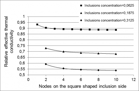
The important point is the choice of the computational grid step which is related to the inclusion minimum size. To select the grid step limits a special series of calculations was carried out. Effective thermal conductivity calculations for regions with the same inclusions arrangement were made using various computational grids. Grids differed from each other by nodes number k, which were positioned on one side of the square shaped inclusion. Here and below, we chose ratio $\frac{\lambda_{i n c}}{\lambda_{m x}}=0,0484$ , which approximately corresponded to the ratio of expanded polystyrene and cement-sand mixture thermal conductivities and temperature difference from θl = 1 to θr = 0,867, that approximately corresponded to temperature reduction from 300 to 260K. Figure 2 illustrates typical results of such calculation series. Figure 2 shows that when $k \subset[1-3]$ the calculation results vary with grid step decreasing and these differences reach 5% at various inclusions predetermined concentrations. Value k should be at least 5 to ensure the calculation accuracy better than 1%. For k > 10 the calculations slightly (less than 0.5%) depend on the number of grid nodes on one side of the square-shaped inclusion.
Figure 2. Calculated dependence $\kappa(k)$ for different inclusions concentration η
3.1 Effective thermal conductivity distribution
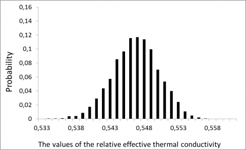
Inclusions random arrangement in the matrix leads to scatter in the heat flux values and therefore to scatter in the values of effective thermal conductivity. Typical probability distribution of the relative effective thermal conductivity values is shown in Figures 3.1 – 3.3. When constructing these histograms, the range of the relative effective thermal conductivity variation in each test series was divided into 28 equal intervals.
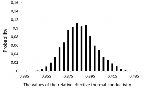
From Figure 3.1 it is seen that for a given ratio of thermal conductivities of the matrix and the inclusions obtained distributions at low concentration of isolated inclusions have negative skewnesses (distributions left wings are more extended) and positive kurtosis (distributions maxima are more sharp than normal distribution maximum). While increasing the inclusions concentration the skewnesses and kurtosis distributions approach zero. Consequently, the distribution becomes more similar to a normal distribution (see Figure 3.2). Then, while further inclusions concentration increasing skewness becomes positive (the distribution extends to the right) and the distribution maximum becomes more blurred (see Figure 3.3).
Figure 3.1. The probability distribution of the composite relative effective thermal conductivity values in the case of isolated inclusions filling; the inclusions concentration η2 = 0,0625; 8000 tests
Figure 3.2. The probability distribution of the composite relative effective thermal conductivity values in the case of isolated inclusions filling; the inclusions concentration η2 = 0,3125; 8000 tests
Figure 3.3. The probability distribution of the composite relative effective thermal conductivity values in the case of isolated inclusions filling; the inclusions concentration η5 = 0,4395; 9000 tests.
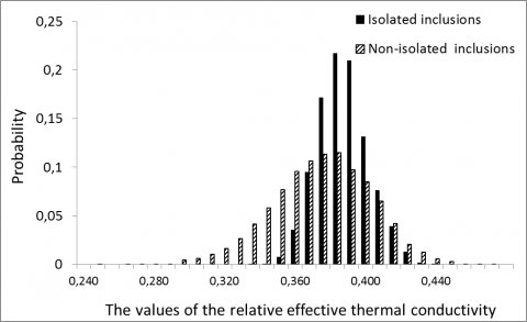
In case of non-isolated inclusions, the distribution scatter increases and distributions left wing is more extended (see Figure 4). In Figure 4 the same distribution as in Figure 3.3 for isolated inclusions (but with a different partition into intervals) is shown to compare them. In Figure 4 partition into intervals is changed to compare with the distribution for non-isolated inclusions more conveniently.
Figure 4. Comparison of probability distributions of composite relative effective thermal conductivity when filling isolated and non-isolated inclusions η5 = 0,4395; 9000 tests
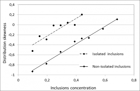
Typical dependences of distribution skewness α3 and kurtosis α4 of the effective thermal conductivity on inclusions concentration $\eta_{5}$ are shown in Figure 5.1 and Figure 5.2 for non-isolated inclusions and isolated inclusions with characteristic size β5 = 5/32; each point on the graph is obtained by at least 4000 tests.
Figure 5.1. The dependence of distribution skewness of the effective thermal conductivity on inclusions concentration $\eta_{5}$ for non-isolated inclusions and isolated inclusions
Figure 5.2. The dependence of distribution kurtosis of the effective thermal conductivity on the inclusions concentration $\eta_{5}$ for non-isolated inclusions and isolated inclusions
The above graphs show that growth of distribution skewness α3 for increasing concentration $\eta_{5}$ can be approximated by a linear dependence. In this case for isolated inclusions $\alpha_{3} \approx 1,758 \cdot \eta_{5}-0,575$; for non-isolated inclusions $\alpha_{3} \approx 1,755 \cdot \eta_{5}-1,085$ . It is interesting that growth rates of the skewness for non-isolated and isolated inclusions are almost equal, but for non-isolated inclusions α3 is on average two times less than for isolated ones. This is true for skewnesses for other characteristic dimensions of inclusions. Kurtosis distribution (see Figure 5.2) varies approximately inversely proportional to the concentration of inclusions.
However, in order to reliably establish the kurtosis dependence on concentration and non-contacted inclusions presence, it is necessary not less than 20000 tests. Unfortunately, we did not have such possibility.
3.2 Effective thermal conductivity concentration dependences
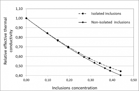
According to the models [5-7], the effective thermal conductivity of the two-phase composite depends only on the phase concentration and density [12] and does not depend on the inclusions placement peculiarities. The calculations show that this statement is true only in the first approximation. Average effective thermal conductivity $\overline{\boldsymbol{K}}$ for non-isolated inclusions is slightly less (up to 5%) than $\overline{\boldsymbol{K}}$ for isolated inclusions when their concentrations are equal. Dependencies $\overline{\boldsymbol{K}}$ on isolated and non-isolated inclusions concentration with characteristic size β5 = 5/32 are shown in Figure 6. Each point on the graph is obtained by at least 4000 tests.
Figure 6. The dependence of average relative effective thermal conductivity on the concentrations for isolated and non-isolated inclusions with characteristic size β5 = 5/32
As can be seen, the dependencies shown in Figure 6 are nonlinear. They are quite well approximated by functions
$\kappa=1-\frac{a \eta}{\sqrt{(1+b \eta)^{3}}}$ (5)
where η is inclusions concentration; a and b are fitting coefficients. Fitting coefficients for isolated inclusions with characteristic size β5 = 5/32 are a ≈ 1,676 and b ≈ 1,115 and for non-isolated inclusions of the same characteristic size are a ≈ 1,679 and b ≈ 0,797. Fitting coefficient a with high accuracy is the same for both types of inclusion.
Investigation of inclusions placement images showed that average effective thermal conductivity in the case of non-isolated inclusions is less than in case of isolated inclusions. This reduction is associated with the proportion of non-isolated inclusions which contact with each other and with minimum layer thickness of the matrix material around the isolated inclusions. The average effective thermal conductivity reduction in the case of non-isolated inclusions can be explained by increasing of the heat flux effective length through the heat-conducting matrix.
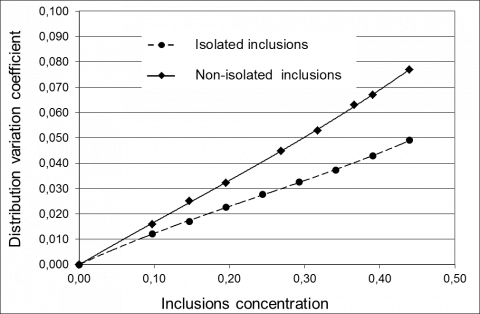
As a measure of the effective thermal conductivity dispersion obtained during different tests, we used the distribution variation coefficient $\vartheta$ . Dependence of distribution variation coefficient $\vartheta$ on inclusions concentration with characteristic size β5 = 5/32 is shown in Figure 7.
Figure 7. Dependences distribution variation coefficient on inclusions concentration for isolated and non-isolated inclusions with a characteristic size β5 = 5/32
The linear dependence $\vartheta=\vartheta\left(\eta_{5}\right)$ allows to describe the distributions broadening of effective relative thermal conductivity with inclusion concentration increasing by parameter $v=\frac{d \vartheta}{d \eta_{5}}$. For isolated inclusions value of $v$ ( $v_{i s l}$ ) is 0,11 and for non-isolated inclusions value of $v$ ( $\mathcal{U}_{\text {noisl }}$ ) is 0,17. Estimates show that the average numbers of inclusions placements in the region bounded by the nearest neighbors for a pattern with concentration $\eta$ isolated and non-isolated inclusions are equal respectively: $W_{i s l}=\left(\frac{k K}{K \sqrt{\eta}+k}-(2 d+1) k\right)^{2}$ , $W_{\text {noisl}}=\left(\frac{k K}{K \sqrt{\eta}+k}-k\right)^{2}$ , where d is the minimum distance between the isolated inclusions. The number of available placements for isolated inclusions is less than for non-isolated: $W_{i s l}<W_{n o i s l}$ . Accordingly, the distribution variation of the effective relative thermal conductivity for heat-isolated inclusions less than for non-isolated inclusions: $v_{i s l}<\mathcal{v}_{\text {noisl}}$ .
1.The paper presents the concentration dependences of the mean value, coefficient of variation, skewness and kurtosis of the effective relative thermal conductivity distribution in the cases of isolated and non-isolated inclusions.
2.It is shown that in the case of non-isolated inclusions the effective thermal conductivity of the material is reduced and the values scatter of the effective thermal conductivity increases. This fact is meaningful to consider in the composite materials manufacturing technology development.
3.It has been found that non-isolated inclusions increase the probability of obtaining a composite material with better heat-insulating properties.
|
K |
square pattern size, grid cells |
|
M |
computational grid size along y-coordinate, grid cells |
|
N |
computational grid size along x-coordinate, grid cells |
|
T |
absolute temperature, K |
|
W |
average numbers of inclusions placements in the region bounded by the nearest neighbors |
|
a |
dimensionless fitting coefficient |
|
b |
dimensionless fitting coefficient |
|
d |
minimum distance between the isolated inclusions, grid cells |
|
i |
computational grid cell number along y-coordinate |
|
j |
computational grid cell number along x-coordinate |
|
k |
square inclusion size, grid cells |
|
n |
number of inclusions, which fell into a pattern |
|
p |
probability |
|
x |
coordinate |
|
y |
coordinate |
|
Greek symbols |
|
|
3 |
distribution skewness |
|
α4 |
distribution kurtosis |
|
β |
dimensionless inclusion size |
|
η |
dimensionless inclusions concentration |
|
θ |
dimensionless temperature |
|
κ |
dimensionless thermal conductivity |
|
λ |
thermal conductivity, W.m-1. K-1 |
|
ν |
number of tests |
|
ξ |
half-width the range of values. |
|
σ |
distribution standard deviation |
|
υ |
dimensionless parameter of the concentration dependence of the thermal conductivity distribution variation |
|
ϑ |
distribution variation coefficient |
|
Subscripts |
|
|
b |
bottom |
|
Ch |
characteristic |
|
inc |
inclusion |
|
isl |
isolated |
|
l |
left |
|
m |
index, which enumerated the range of relative thermal conductivity values |
|
mx |
matrix |
|
noisl |
non-isolated |
|
r |
right |
|
t |
top |
[1] Boulaoued I., AmAra I., Mhimid A. (2016). Experimental determination of thermal conductivity and diffusivity of new building insulating materials, International Journal of Heat and Technology, Vol. 34, No. 2, pp. 325-331. DOI: 10.18280/ijht.34024
[2] McCullough R.L. (1985). Generalized combining rules for predicting transport properties of composite materials, Compos. Sci. Technol., Vol. 22, No. 1, pp. 3-21. DOI: 10.1016/0266-3538(85)90087-9
[3] Simpkin R. (2010). Derivation of Lichteneckers’s logarithmic mixture formula from Maxwell’s equations, IEEE Trans. Microw. Theory Techn., Vol. 58, No. 3, pp. 545-550. DOI: 10.1109/TMTT.2010.2040406
[4] Ganapathy D., Singh K., Phelan P.E., Prasher R. (2005). An effective unit cell approach to compute the thermal conductivity of composites with cylindrical particles, J. Heat Transfer, Vol. 127, No. 6, pp. 553-559. DOI: 10.1115/1.1915387
[5] Pietrac K., Wiśniewski T.S. (2015). A review of models for effective thermal conductivity of composite materials, Journal of Power Technologies, Vol. 95, No. 1, pp. 14-24. Available: http://papers.itc.pw.edu.pl/index.php/JPT/article/view/463/637
[6] Pradhan N.R., Iannacchione G.S. (2010). Thermal properties and glass transition in PMMA+SWCNT composites, J. Phys. D: Appl. Phys., Vol. 43, No. 30, pp. 305-403. DOI: 10.1088/0022-3727/43/30/305403
[7] Baziuk L.V., Sirenko H.A. (2013). Thermophysical properties of metals and polymer compositions (review), Physics and Chemistry of Solid State, Vol. 14, No. 1, pp. 21-27. Available: www.pu.if.ua/inst/phys_che/start/pcss/vol14/1401-02.pdf
[8] Nikitin A.V., Liopo V.A., Avdeichuk S.V., Struk V.A. (2014). Model representations of thermal conductance in polymer nanocomposites, Belgorod State University Scientific Bulletin Mathematics & Physics, Vol. 5(176), No. 34, pp. 150-160. Available: www.bsu.edu.ru/upload/iblock/fc0/NOM1(2014).pdf
[9] Fedotovsky V.S., Orlov A.I. (2008). The effective thermal conductivity of the bundles of rods and pipes in their random deviations from the regular lattice, Izvestia Vysshikh Uchebnykh Zawedeniy. Yadernaya Energetika, No 4, pp. 113-120. Available: http://journal.iate.obninsk.ru/sites/default/files/Number4%282008%29.pdf
[10] Devpura A., Phelan P.E., Prasher R.S. (2001). Size effects on the thermal conductivity of polymers laden with highly conductive filler particles, Microscale Thermophys. Eng., Vol. 5, No. 3, pp. 177-189. DOI: 10.1080/108939501753222869
[11] Bakshi S.R., Patel R.R., Agarwal A. (2010). Thermal conductivity of carbon nanotube reinforced aluminum composites: a multi-scale study using object oriented finite element method, Comput. Mater. Sci., Vol. 50, No. 2, pp. 419-428. DOI: 10.1016/j.commatsci.2010.08.034
[12] Baccilieri F., Bornino R., Fotia A., Marino C., Nucara A., Pietrafesa M. (2016). Experimental measurements of the thermal conductivity of insulant elements made of natural materials: preliminary results, International Journal of Heat and Technology, Vol. 34, No. Sp. 2, pp. S413-S419. DOI: 10.18280/ijht.34Sp0231