OPEN ACCESS
Supersonic ejectors can be used in heat powered chillers to transfer mechanical energy between the motive and the inverse cycle. Within the ejector, momentum is exchanged between a high speed flow produced by a primary nozzle and a slow current coming from the chiller evaporator. Due to the supersonic regime of the primary flow, the mixing of the two streams causes significant loss and impairs the system efficiency. Up to now, second law efficiency of ejector chillers is quite low and optimization is highly needed. The fluid dynamics of the whole ejector involves turbulent mixing, shock trains and complex wall flow, requiring CFD analyses for an adequate description. However, in order to attempt an optimization, mathematically workable models are advantageous.
An analytical scheme that captures the basic features of the turbulent mixing zone is discussed here in view of a Constructal design of an ejector chiller.
Supersonic ejector chiller, Compressible turbulent mixing, Mixing layer model, Second law analysis, Constructal design.
Supersonic ejectors are passive compression devices that are employed for a range of applications, from aeronautic high-speed propulsion systems to the compression of refrigerants in energy and refrigeration systems. In particular, the use of ejectors in refrigeration applications is a promising solution in the light of its ability to exploit low temperature heat to produce cooling. Unfortunately, ejector refrigerators are still quite far from the performance obtained by absorption cycle machines, mostly due to the severe losses occurring inside the supersonic ejector. Even so, the common practice is to design the ejector according to empirical prescriptions (e.g. ESDU [1]) or to use simplified models to compute the main geometric characteristics. These methods are generally inadequate for thermodynamic optimization, as they are unable to predict the system efficiency as a function of its design. In most cases, models overlook the dynamics of turbulent mixing and only consider global momentum balances adjusted through simple efficiency parameters. Yet, turbulent mixing is arguably the most important process occurring inside ejectors, as it determines the amount of suction flow entrainment and a considerable share of the system’s total thermodynamic losses. In what follows, an analytical scheme that captures the basic features of the turbulent mixing zone is discussed. The model builds on a previous scheme devised by Papamoschou [1-2] and is able to compute all flow properties inside an axisymmetric or planar mixing chamber with either constant or variable cross section. The amount of secondary flow entrainment, the work and heat exchange, pressure losses and mixing efficiency are computed as a function of the system geometry and without use of any arbitrary parameter. Consequently, this model is particularly suited for a thermodynamic optimization of the ejector system.
The model will be validated by comparison with CFD results for various operating conditions. Furthermore, its use as a tool for a Constructal design of the ejector chiller will be discussed.
When the primary and secondary flow meet inside the mixing chamber, they give rise to a narrow region of strong mixing called “mixing layer”. Most interestingly, turbulence inside the mixing layer is not homogeneous but rather characterized by the formation of coherent eddies which were first revealed by the work from Brown and Roshko [4]. There are many theories explaining the birth and dynamics of these structures (see for example [5] or [6]) and the interested reader may refer to those for more details on this subject. From the point of view of supersonic ejectors, we are interested in the more specific case of compressible mixing layers, whose main problems are well illustrated in monographs like those from Smits and Dussauge [7] and Gatsky and Bonnet [8].
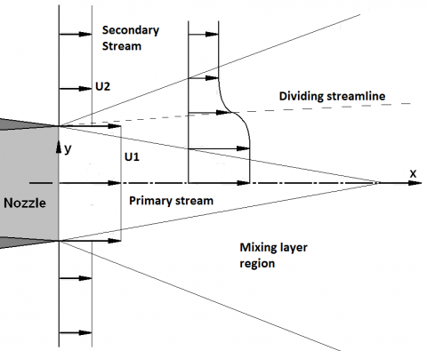
Figure 1 shows the main features of a mixing layer. Outside this region the primary (motive) and secondary (suction) streams flow isentropically. Inside the mixing layer, the time averaged velocity smoothly varies from the value of the undisturbed primary stream to that of secondary stream. The extension of the shear region is usually measured by the definition of a “shear layer thickness”. In general, there are many ways to define this quantity that, unfortunately, are not completely equivalent and can lead to difficulties in the comparison of experimental data [8]. In what follows, only one of these will be considered, i.e., the “vorticity thickness”.
Figure 1. Mixing layer inside an ejector
The vorticity thickness is defined as the distance given by the ratio of the velocity difference across the layer divided by the maximum slope of the velocity profile:
$\delta_{\omega}=\Delta U_{\infty} /\left(\frac{\partial U}{\partial y}\right)_{\max }$(1)
where ΔU∞ is the difference between the undisturbed primary and secondary stream velocities.
This definition is most useful whenever an analytical function that approximates the mixing layer velocity profile is provided. For instance, if the velocity is described by a hyperbolic tangent, the knowledge of the vorticity thickness allows exact definition of the mixing layers edges. The spreading rate of the shear layer thickness along the axial direction is defined as:
$\delta_{\omega}^{\prime}=\frac{d \delta_{o}}{d x}$(2)
An interesting feature of most shear flows (jets, mixing layers, and wakes) is that the spreading rate of the shear layer (eq. 2) is constant, i.e. the shear region grows linearly with distance (see fig. 1).
Experimental investigations performed in the 70s have shown that compressible mixing layers are affected by a significant reduction of the mixing layer spreading rate with respect to low speed flows ([4], [9]). The causes of this phenomenon have been the subject of studies for more than 50 years, and yet no clear explanation has been found. Early studies tried to explain the effect by the density variations resulting from the high expansion levels. However, the work of Brown and Roshko [4] demonstrated that this was not the main cause. Papamoschou and Roshko [10] later found that the decrease of mixing layer spreading rate may be described by means of a parameter called convective Mach number:
$M_{c}=\frac{\Delta U_{\infty}}{a_{\infty 1}+a_{\infty 2}}$(3)
where a∞1 and a∞2 are the sound speed of the primary and secondary stream outside the mixing layer.
The use of the convective Mach number allows approximate correlation of the experimental data of compressible mixing layer spreading rates. Among the several correlations, one of the most simple and popular was provided by Papamoschou and Roshko [10] and later readapted by Papamoschou [2-3]:
$\delta_{\omega}^{\prime}=\delta_{\omega_{-i n c o m p}}^{\prime} \cdot f\left(M_{c}\right)=0.085 \cdot\left[\frac{(1+\eta)(1-r)}{(1+r \eta)}\right] \cdot f\left(M_{c}\right)$(4)
where $\eta=\sqrt{\rho_{\infty 2} / \rho_{\infty 1}}, r=U_{\infty 2} / U_{\infty 1}$; the compressibility function is defined as the ratio of the compressible to incompressible spreading rate, and is given by:
$f\left(M_{c}\right)=\frac{\delta_{\omega}^{\prime}}{\delta_{\omega_{-} i n c o m p}^{\prime}} \approx 0.25+0.75 e^{-3 M_{c}^{2}}$(5)
The terms inside square brackets in eq. 4 describe the effect of density and velocity difference across the layer, which is to increase the spreading rate for large velocity differences and when the density is greater on the low speed side. The effect of compressibility is concentrated in the exponential function (eq. 5) and brings about a significant reduction in the mixing layer spreading rate.
Equation 4 provides a mean to easily calculate the spreading rate by the knowledge of flow conditions in the isentropic region outside the layer. Unfortunately, eq. 5 shows discrepancies of the order of 20% or more with respect to experimental data [2]. The main reason for this large uncertainty is to be found in the scatter of most experimental data. In general, mixing layers are influenced by blockage effects, thickness and surface conditions of the splitter plate, inlet turbulence level and acoustic effects [7]. These effects cannot be captured by the sole use of eq. 5 and greater accuracy may be achieved by the introduction in eq. 4 of some further parameters accounting for these additional factors.
Lastly, the knowledge of the spreading rate allows deriving a fundamental equation for the maximum shear stress inside the mixing layer. By means of dimensional arguments it can be demonstrated that the maximum shear stress is approximately given by [2]:
$\tau_{\max } \sim \frac{d \delta_{\omega}}{d x} \rho_{a v g} U_{a v g} \Delta U_{\infty}$$=K \cdot \frac{1}{2}\left(\rho_{\infty 1}+\rho_{\infty 2}\right) \Delta U_{\infty}^{2}\left[\frac{(1+\eta)(1+r)}{2(1+r \eta)}\right] \cdot f\left(M_{c}\right)$(6)
where K is an empirical constant, obtained from subsonic constant-density experiments. Papamoschou [2-3] suggests use of Wygnanski and Fiedler's value, K = 0.013 [11].
In order to exploit the information on the maximum shear stress, the location where this stress is exchanged must be known. Townsend [12] showed that the maximum shear stress inside a constant pressure mixing layer occurs approximately on the dividing streamline, i.e., the line that divides two fluid regions having mass flow rates equal to that of primary and secondary stream. The division is purely virtual, in that the two streams actually mix and do not preserve their identities. Nonetheless, the knowledge of the density and velocity profiles along the ejector cross section allows computation, for any axial position, of the height or radius that separates these two regions.
The knowledge of the location of the dividing streamline will be mostly useful in the development of the present model, as illustrated in the following section.
The model analyses the primary and secondary stream separately by applying the conservation equations on two control volumes that surround each stream. To this aim, the position of the dividing streamline is computed at each step by requiring pressure continuity across it, i.e., by imposing that the pressure of primary and secondary stream are equal at each cross section. Under this condition, the primary nozzle flow is correctly expanded and the intensity of expansions and shock trains (shock diamonds) are reduced, increasing mixing effectiveness and reducing pressure losses ([9], [13]). The shear stress, shear work and heat transfer across the dividing streamline, as well as friction at wall, are computed by means of experimental correlations. Both axisymmetric and planar configurations can be studied.
The mixing layer flow inside a supersonic ejector is well approximated by the 2D compressible boundary layer equations [14]. For the planar case, it could be shown by dimensional arguments that these reduce to [7]:
$\frac{\partial \overline{\rho} \tilde{u}}{\partial x}+\frac{\partial \overline{\rho} \tilde{v}}{\partial y}=0$
$\overline{\rho} \tilde{u} \frac{\partial \tilde{u}}{\partial x}+\overline{\rho} \tilde{v} \frac{\partial \tilde{u}}{\partial y}=-\frac{\partial \overline{p}}{\partial x}+\frac{\partial \tau}{\partial y}$
$\overline{\rho} \tilde{u} \frac{\partial \tilde{h}_{0}}{\partial x}+\overline{\rho} \tilde{v} \frac{\partial \tilde{h}_{0}}{\partial y}=\frac{\partial}{\partial y}[w+q]$(7)
Where the straight bars over the symbols indicate a Reynolds average while the tilde a Favre average; τ, w and q are respectively the total (i.e., viscous plus turbulent) shear stress, shear work (per unit time and area) and heat transfer:
$\tau=\tau_{v}+\tau_{t}=\left(\mu+\mu_{t}\right) \frac{\partial \tilde{u}}{\partial y}=\mu \frac{\partial \tilde{u}}{\partial y}+\tilde{u} \overline{\rho u^{\prime} v^{\prime}}$
$w=w_{v}+w_{t}=\tilde{u} \cdot\left(\tau_{v}+\tau_{t}\right)=\tilde{u} \cdot \mu \frac{\partial \tilde{u}}{\partial y}+\tilde{u}^{2} \overline{\rho u^{\prime} v^{\prime}}$
$q=q_{v}+q_{t}=\left(k+k_{t}\right) \frac{\partial \tilde{T}}{\partial y}=k \frac{\partial \tilde{T}}{\partial y}+C_{p} \overline{\rho T^{\prime} v^{\prime}}$(8)
where the heat and momentum transfer by turbulent fluctuations are expressed as a function of the average velocity and temperature gradients through the definition of a turbulent viscosity and conductivity (Boussinesq approximation).
Generally, for shear layers far from any solid wall (such as mixing layers, jets and wakes) it is customary to neglect the viscous effects. However, in building the mixing layer model for the ejector, and especially for the secondary stream, the viscous drag at wall must be included.
As anticipated, a system of Quasi-One-Dimensional conservation equations will be applied separately to each of the two streams. Although the flow inside an ejector cannot be considered as 1D, the 2D effects are retained by the use of two corrective parameters that will be introduced later. The use of Q1D approximation brings about many benefits: first, it provides for a set of equations that can be solved in a much easier way than the “integral methods” needed to compute the full 2D equations (see for example [15-16]); second, it allows for an easy connection with primary nozzle and diffuser equations (as these regions can legitimately be regarded as Q1D) to build a compact and coherent model of the complete ejector; last, by means of the Q1D approximation, the ejector can be seen as an equivalent “momentum exchanger” and many interesting conclusion can be drawn about the thermodynamic optimization of the system (see section 6).
In order to derive the Q1D equations, equations 7 must be integrated over the cross sectional area:
$\int_{A}\left(\frac{\partial \overline{\rho} \tilde{u}}{\partial x}+\frac{\partial \overline{\rho} \tilde{v}}{\partial y}\right) d A=0$
$\int_{A}\left(\overline{\rho} \tilde{u} \frac{\partial \tilde{u}}{\partial x}+\overline{\rho} \tilde{v} \frac{\partial \tilde{u}}{\partial y}\right) d A=\int_{A}\left(-\frac{\partial \overline{p}}{\partial x}+\frac{\partial \tau}{\partial y}\right) d A$
$\int_{A}\left(\overline{\rho} \tilde{u} \frac{\partial \tilde{h}_{0}}{\partial x}+\overline{\rho} \tilde{v} \frac{\partial \tilde{h}_{0}}{\partial y}\right) d A=\int_{A} \frac{\partial}{\partial y}[w+q] d A$(9)
The continuity equation is exploited to rearrange the equations in conservative form. In addition, all the equations are divided by the ejector depth (which is constant) to integrate over the sole y coordinate:
$\int_{y}\left(\frac{\partial \overline{\rho} \tilde{u}}{\partial x}+\frac{\partial \overline{\rho} \tilde{v}}{\partial y}\right) d y=0$
$\int_{y}\left(\frac{\partial \overline{\rho} \tilde{u}^{2}}{\partial x}+\frac{\partial \overline{\rho} \tilde{v} \tilde{u}}{\partial y}\right) d y=\int_{y}\left(-\frac{\partial \overline{p}}{\partial x}+\frac{\partial \tau}{\partial y}\right) d y$
$\int_{y}\left(\frac{\partial \overline{\rho} \tilde{u} \tilde{h}_{0}}{\partial x}+\frac{\partial \overline{\rho} \tilde{v} \tilde{h}_{0}}{\partial y}\right) d y=\int_{y} \frac{\partial}{\partial y}[w+q] d y$(10)
The continuity equation can be transformed as follows:
$\int_{y} \frac{\partial \overline{\rho} \tilde{u}}{\partial x} d y+\int_{y} \frac{\partial \overline{\rho} \tilde{v}}{\partial y} d y=\frac{d}{d x} \int_{y} \overline{\rho} \tilde{u} d y+[\overline{\rho} \tilde{v}]_{y_{i}}^{y_{e}}$(11)
where the Leibniz rule was used to extract the derivatives from the first term on the RHS. The second term must be integrated between the internal and external surface surrounding each stream, i.e., between the axis of symmetry and the dividing streamline for the primary stream and between the dividing streamline and the ejector shroud for the secondary stream. In all cases, the mass fluxes across these surfaces are zero and the second term on the RHS vanishes.
Thus, after multiplying back by the ejector depth, the Q1D equation of continuity becomes:
$d(\langle\overline{\rho}\rangle\langle\tilde{u}\rangle A)=0$(12)
where the terms in angle brackets are the “spatially averaged” velocity and density:
$\langle\widetilde{u}\rangle=\frac{\int_{y} \overline{\rho} \widetilde{u} d y}{\int_{y} \overline{\rho} d y}$ $\langle\overline{\rho}\rangle=\frac{\int_{y} \overline{\rho} d y}{\int_{y} d y}$(13)
The momentum equation becomes:
$\frac{d}{d x} \int_{y} \overline{\rho} \tilde{u}^{2} d y+[\overline{\rho} \tilde{v} \tilde{u}]_{y_{i}}^{y_{e}}=-\frac{d \overline{p}}{d x}+[\tau]_{y_{i}}^{y_{e}}$(14)
where pressure was assumed uniform in the transversal direction. As seen for the continuity equation, the second term on the LHS is zero. The term containing the shear stress depends on the position where the integration is performed.
The Q1D momentum equation finally reads:
$d\left(\langle\overline{\rho}\rangle\left\langle\tilde{u}^{2}\right\rangle A\right)+d \overline{p}=\left(\tau_{e}-\tau_{i}\right) d S$(15)
where the “spatially averaged squared velocity” is defined as:
$\left\langle\tilde{u}^{2}\right\rangle=\frac{\int_{y} \overline{\rho} \tilde{u}^{2} d y}{\int_{y} \overline{\rho} d y}$(16)
It is now easy to show that the Q1D energy equation is given by:
$d\left(\langle\overline{\rho}\rangle\left\langle\tilde{u}^{3}\right\rangle A\right)+d(\langle\overline{\rho}\rangle\langle\tilde{u}\rangle\langle\tilde{h}\rangle A)=\left(w_{e}+q_{e}\right) d S-\left(w_{i}+q_{i}\right) d S$(17)
where the “spatially averaged total enthalpy” and “spatially averaged cubed velocity” are defined by:
$\langle\tilde{h}\rangle=\frac{\int \overline{\rho} \tilde{u} \tilde{h} d y}{\int_{y} \overline{\rho} \tilde{u} d y}$ $\left\langle\tilde{u}^{3}\right\rangle=\frac{\int \overline{\rho} \tilde{u}^{3} d y}{\int_{y} \overline{\rho} d y}$(18)
To summarize, the Q1D equations are as follows:
$d(\rho\langle u\rangle A)=0$
$d\left(\rho\left\langle u^{2}\right\rangle A\right)+d \overline{p}=\left(\tau_{e}-\tau_{i}\right) d S$
$d\left(\rho\left\langle u^{3}\right\rangle A\right)+d(\rho\langle u\rangle h A)=\left(w_{e}+q_{e}\right) d S-\left(w_{i}+q_{i}\right) d S$(19)
In the last equations all the average symbols have been dropped except those related to the average velocities. In this form, equations 19 clearly show what the unknowns of the problem are. In particular, two additional variables appear, i.e. the averaged squared and cubed velocities that do not allow closure of the equations system. In order to overcome this problem, two “shape coefficients” may be defined as follows:
$\alpha=\frac{\left\langle u^{2}\right\rangle}{\langle u\rangle^{2}}=\frac{\int_{y} \overline{\rho} \tilde{u}^{2} d y}{\int_{y} \overline{\rho} d y} \cdot\left[\frac{\int_{y} \overline{\rho} d y}{\int_{y} \overline{\rho} \tilde{u} d y}\right]^{2}$(20a)
$\beta=\frac{\left\langle u^{3}\right\rangle}{\langle u\rangle^{3}}=\frac{\int_{y} \overline{\rho} \tilde{u}^{3} d y}{\int_{y} \overline{\rho} d y} \cdot\left[\begin{array}{c}{\int_{y} \overline{\rho} d y} \\ {\int_{y} \overline{\rho} \tilde{u} d y}\end{array}\right]^{3}$(20b)
In the simple case of a uniform velocity profile, i.e. for 1D flow, the average velocity can be taken out of the integrals and the shape coefficients become equal to one. However, such approximation is only valid in certain kind of flow, most importantly for fully developed turbulent flow inside constant section channels (as long as the small non uniformities due to the boundary layer are neglected) or in channels with slow area variations (e.g. Q1D flows). Unfortunately, the approximation is no longer valid in case of large non uniformity of the velocity profiles due to the presence of shear flows like mixing layers, jets and wakes. In these cases the flow is actually 2D but the problem may be worked around by the use of the above defined “shape coefficients”. By introduction of these parameters, the governing equations become:
$d m=0$
$m d(\alpha u)+d \overline{p}=\left(\tau_{e}-\tau_{i}\right) d S$
$m d\left(\beta u^{2}+h\right)=\left(w_{e}+q_{e}\right) d S-\left(w_{i}+q_{i}\right) d S$(21)
where m is the mass flow rate which is constant for each stream.
If the variation of the velocity profile is slow enough, the two shape coefficients can be considered approximately constant along a distance dx. This allows taking out the shape coefficients from the differentials. The coefficients will nevertheless be updated at the end of each calculation step. Moreover, by considering a calorically and thermally perfect gas, equations 21 can be assembled into two equations for the velocity and Mach variation:
$\frac{d U}{U}=\frac{1}{\phi_{1}}\left[\frac{d A}{A}+\frac{d x}{p}\left(\frac{\tau_{i}}{l_{i}}+\frac{\tau_{e}}{l_{e}}\right)-\frac{(\gamma-1)}{\gamma} \frac{d x}{p U}\left(\frac{q_{i}+w_{i}}{l_{i}}+\frac{q_{e}+w_{e}}{l_{e}}\right)\right]$
$\frac{d M}{M}=\frac{\phi_{2}}{\phi_{1}}\left[\frac{d A}{A}+\frac{d x}{p}\left(\frac{\tau_{i}}{l_{i}}+\frac{\tau_{o}}{l_{e}}\right)\right]-\frac{2 \phi_{2}+\phi_{1}}{2 \phi_{1}}\left[\frac{\gamma-1}{\gamma} \frac{d x}{p U}\left(\frac{q_{i}+w_{i}}{l_{i}}+\frac{q_{e}+w_{e}}{l_{e}}\right)\right]$(22)
where the signs of the terms inside round brackets must be adjusted for each stream according to the specific boundary conditions. In eq. 22, lx is the ratio between the cross sectional area and the wetted perimeter of the surface x. The two coefficients φ1 and φ2 depend solely on Mach number and shape coefficients, and are given by:
$\phi_{1}=\left(M^{2}(1+\alpha-\beta)-1\right)$
$\phi_{2} \equiv 1+\frac{(\gamma-1)}{2} \beta M^{2}$(23)
In order to calculate eq. 22 the shape coefficients, area variation, shear stress, shear work and heat transfer must be known on each surface surrounding the primary and secondary stream.
Following Papamoschou [2], the shear stress at wall is computed through Van Driest correlation for compressible boundary layer on smooth walls [14]:
$0.242 \sqrt{\frac{1-\lambda^{2}}{c_{f}}} \frac{\sin ^{-1}(\lambda)}{\lambda}=\log _{10}\left(\operatorname{Re}_{x} c_{f}\right)+1.26 \log _{10}\left(1-\lambda^{2}\right)$
$1-\lambda^{2}=\left(1+\frac{\gamma-1}{2} M_{\infty}^{2}\right)^{-1}$(24)
where Rex is the Reynolds number based on streamwise distance x and cf is the skin friction coefficient. The wall shear stress is computed as follows:
$\tau_{w}=c_{f} \frac{1}{2} \rho_{\infty} U_{\infty}^{2}$(25)
The shear stress on the dividing streamline is computed by means of eq. 6.
In order to compute the heat transfer across the dividing streamline, the turbulent Prandtl number may be introduced as follows:
$P_{t}=\frac{\mu_{t} C_{p}}{k_{t}}$(26)
where μt and kt are the turbulent dynamic viscosity and conductivity. Cp is the specific heat capacity at constant pressure.
A major simplification is obtained by considering that the turbulent Prandtl number is unity. This is known as Strong Reynolds Analogy (SRA) and amounts to say that the heat and momentum transfer by turbulent fluctuations are driven by the same transport mechanisms. In case of mixing layers, a better approximation is to consider Pt ≈ 0.77 ([7], [14]). The use of the Reynolds Analogy allows computing the heat transfer by the knowledge of the turbulent shear stress on the dividing streamline:
$q_{t}=\frac{\mu_{t} C_{p}}{P_{t}} \frac{\partial \tilde{T}}{\partial y}=\frac{C_{p}}{0.77} \frac{\partial \tilde{T}}{\partial y} \frac{\partial y}{\partial \tilde{u}} \tau_{t} \approx \frac{C_{p}}{0.77} \frac{\Delta T_{\infty}}{\Delta U_{\infty}} \tau_{t}$(27)
The only terms missing are now the shear work and the shape coefficients. These quantities may be computed once a profile is assumed for the density and velocity inside the mixing layer.
Some experiments have shown that in fully developed mixing layers the shape of the velocity profile is virtually unaffected by compressibility [7-8]. This means that compressibility affects the spreading rate of the layer while maintaining the velocity distribution unaltered. Therefore, it is possible to use fitting curve derived for incompressible flows in order to describe the velocity distribution of the compressible case.
Unfortunately, there are many different possibilities depending on the type of fitting curve (e.g. error function or hyperbolic tangent) and thickness definitions (e.g. vorticity thickness, velocity thickness, etc…). Barone et al. [17] made a clear comparison of many of these different solutions. One of these exploits a hyperbolic tangent distribution based on the vorticity thickness:
$\frac{U_{s l}-U_{\infty 2}}{U_{\infty 1}-U_{\infty 2}}=\frac{1}{2}\left[1+\tanh \left(2.002 \cdot \frac{y-y_{0}}{\delta_{\omega}}\right)\right]$(28)
Where y0 is the mixing layer centerline, i.e., the location where the velocity is equal to the average of the two external isentropic velocities.
In order to reach workable formulations for the shear work and shape coefficients, we make a further simplification and consider a linear approximation of the hyperbolic tangent profile (that corresponds to the first order truncation of the Taylor expansion):
$U_{s l} \approx U_{\infty 2}+\frac{\Delta U_{\infty}}{2}\left(1+2.002 \cdot \frac{y-y_{0}}{\delta_{\omega}}\right) \approx U_{\infty_{-} a v e}+\frac{\Delta U_{\infty}}{\delta_{\omega}} y$(29)
where it was assumed that the origin of the coordinate system is on the mixing layer centerline and that the primary flow lies below the longitudinal axis.
For a linear profile, the derivates of the axial velocity along the mixing layer is constant and the vorticity thickness immediately gives an estimation of the shear layer thickness:
$\delta_{o}=\Delta U_{\infty} /\left(\frac{\partial U}{\partial y}\right)_{\max } \approx \Delta Y_{s l}$(30)
By further assuming that the layer spread symmetrically with respect to the position of the dividing streamline, the edges of the mixing layer are found by adding and subtracting one half of the vorticity thickness to the dividing streamline location [3]. Moreover, the velocity at the dividing streamline can be easily computed and the shear work becomes:
$w_{t}=\tilde{u}_{d s l} \tau_{t} \approx U_{\infty_{-} a v g} \tau_{t}=\frac{U_{\infty 1}+U_{\infty 2}}{2} \tau_{t}$(31)
Finally, in order to calculate the shape coefficients, eq. 20, the velocity and density profiles must be computed at each time step. A major simplification is obtained by assuming that the density variation inside the mixing layer is negligible with respect to the velocity variation. Under this condition, the density can be eliminated in eq. 20 and a closed form expression for the shape coefficients can be found. For the planar configuration these are given by:
$\begin{align} & {{\alpha }_{x}}=\frac{\left\langle U_{x}^{2} \right\rangle }{{{\left\langle U_{x}^{{}} \right\rangle }^{2}}}=\frac{4}{3}{{\delta }_{tot\_x}}\frac{\left[ 3U_{\infty \_x}^{2}\left( {{\delta }_{tot\_x}}-{{\delta }_{sl\_x}} \right)+\left( U_{dsl}^{2}+{{U}_{\infty \_x}}{{U}_{dsl}}+U_{\infty \_x}^{2} \right){{\delta }_{sl\_x}} \right]}{{{\left[ 2{{U}_{\infty \_x}}\left( {{\delta }_{tot\_x}}-{{\delta }_{sl\_x}} \right)+\left( {{U}_{dsl}}+{{U}_{\infty \_x}} \right){{\delta }_{sl\_x}} \right]}^{2}}} \\ & {{\beta }_{x}}=\frac{\left\langle U_{x}^{3} \right\rangle }{{{\left\langle U_{x}^{{}} \right\rangle }^{3}}}=2\delta _{tot\_x}^{2}\frac{\left[ 4U_{\infty \_x}^{3}\left( {{\delta }_{tot\_x}}-{{\delta }_{sl\_x}} \right)+\left( U_{dsl}^{3}+U_{dsl}^{2}U_{\infty \_x}^{{}}+U_{dsl}^{{}}U_{\infty \_x}^{2}+U_{\infty \_x}^{3} \right){{\delta }_{sl\_x}} \right]}{{{\left[ 2{{U}_{\infty \_x}}\left( {{\delta }_{tot\_x}}-{{\delta }_{sl\_x}} \right)+\left( {{U}_{dsl}}+{{U}_{\infty \_x}} \right){{\delta }_{sl\_x}} \right]}^{3}}} \\ \end{align}$ (32)
Where x can be either 1 or 2, meaning the primary or secondary flow; δsl is the part of the shear layer thickness related to the primary or secondary stream; δtot represents the total thickness of the primary or secondary flow (isentropic plus shear region).
At the beginning of this chapter, it was mentioned that a basic assumption for the model is that the mixing occurs at constant pressure. This condition is required by many of the correlation presented and is needed to find the position of the dividing streamline (see next section). By further assuming that the density of the two streams is approximately equal, we are implicitly imposing the same inlet static state for the primary and secondary streams. However, this restriction should not be regarded as a mere simplifying assumption, but rather as an optimal operating condition. The only energy exchange that is useful for the purpose of an ejector chiller is the mechanical energy transfer between the primary and secondary stream. By imposing the same static conditions, the entropy generation due to heat transfer mechanism and shock adaptations are reduced to a minimum.
In conclusion, it is important to point out that the need for a shape coefficient derives from the attempt of applying a Q1D model to a flow that is actually 2D. This kind of flow may be solved by use of “integral methods” as long as the profiles of the velocity and of the other quantities are known [15-16]. The method illustrated here can be considered to lie somewhere between a pure Q1D scheme and a 2D integral method.
In the next section we briefly illustrate the calculation procedure for the present model.
The solution method for the mixing layer model quite precisely follows that delineated by Papamoschou [3]. Figure 3 shows the flow chart of the process. Three nested loops are needed to perform the calculation. The outer loops over the inlet static pressure, the intermediate loops over the mixing chamber length and the inner loops over the position of the dividing streamline. A VBA code was written to perform the computations.
The input data for the program are the same as those needed for CFD calculations, i.e., inlet stagnation conditions for both streams (pressure and temperature), outlet static pressure, geometry of the mixing chamber and of primary nozzle, type of fluid and type of symmetry (axial or planar). The output is represented by all flow properties along the mixing chamber as well as the ejector ER, the shear work and heat transfer between primary and secondary stream, the shear stress at wall, the thickness of the mixing layer and many other quantities (see section 5).
As a first step, an initial value for the inlet static pressure must be guessed (equal for both primary and secondary stream). The primary mass flow rate and nozzle exit area are then computed by knowing the primary nozzle throat diameter and by applying the ideal Q1D nozzle equations. The secondary stream inlet area is computed subtracting the primary nozzle exit area to the total mixing chamber area. The secondary mass flow rate and all other properties immediately follow by application of the perfect gas isentropic relations. A first tentative value of ER is computed. The calculation of the mixing chamber can now proceed. The program computes the value of the shear stress at wall and on the dividing streamline, the shear work and heat transfer and the mixing layer spreading rate (eq. 6, 25, 27 and 31). Afterwards, a tentative slope of the dividing streamline is assumed in order to calculate a provisional value of the primary and secondary stream cross sectional areas. The initial value of all the shape coefficients is one, in that the inlet conditions are those of uniform isentropic flow. Hence, the program solves equations 22 for both the primary and secondary stream by means of a fourth order Runge-Kutta procedure. From the ratio of the new velocity to Mach number the programs computes the new sound speed for both stream and calculates the pressure as follows:
$p=\frac{\dot{m} a}{\gamma M A}$(33)
In general, the new pressure will be different for the primary and secondary flow. Hence, the program loops over the slope of the dividing streamline until the pressure difference between the primary and secondary stream is lower than a desired threshold. Once the new pressure is found, all other average properties can be computed easily by exploiting the equation of state and sound speed definition for perfect gases. Afterwards, the program calculates all the properties of the isentropic flow outside the mixing layer by the knowledge of the new static pressure and of the starting stagnation conditions. At this point the program has all the required information to proceed to the next step.
In general, once the program arrives at the end of the mixing chamber, the outlet pressure will differ from that imposed as an input. Hence, the program goes back to the inlet, changes the value of the inlet pressure and loops again over the ejector length. The process goes on until convergence.
Comparison with CFD simulations are performed for a constant area axisymmetric mixing chamber of 0.4 meter length, with a radius of 54 mm. The working fluid is air. The length of the chamber was selected in order to model the sole region of free mixing layer, i.e., the region where the shear layer has reached neither the axis of symmetry nor the mixing chamber wall. In the first case, the primary isentropic region ceases to exist and a “jet type” of flow begins. In the second case, the secondary isentropic region ends and a new flow regime (that we may call “confined mixing layer”) begins. In both cases the Q1D model is unable to compute the shear stress on the dividing streamline (as the isentropic velocities and densities are undefined) and the program stops. Future work will be directed to extend the calculations to these types of flows in order to realize a complete model of the ejector.
Simulations are performed using the commercial CFD package ANSYS FLUENT v15, which is based on a finite volume approach. The details of the numerical scheme, as well as its validation, are described thoroughly in [13]. In brief, the main characteristics of the scheme are as follows:
In addition, a slip wall conditions was imposed at the primary nozzle walls. This is done in order to focus the comparison on the sole mixing zone. As such, both Q1D and CFD primary nozzle expansion are considered completely isentropic. On the contrary, the wall friction along the mixing chamber is evaluated through low Reynolds models for the CFD and by means of eq. 25 for the Q1D model.
Table 1 shows the boundary conditions of the 4 cases tested herein. These were selected in order to guarantee the matching of the static state between the primary and secondary stream. The value of outlet pressure is raised from one case to another in order to test the model with increasingly challenging conditions. In order to correctly compare the results of the Q1D model with those from CFD calculations, a macro was built that extracts the local CFD data for several cross sections. These data are processed to compute the same average quantities that are calculated by the Q1D model.
Table 1. Boundary conditions for the 4 tested cases
|
|
Unit |
Case 1 |
Case 2 |
Case 3 |
Case 4 |
|
T01 - inlet |
°C |
360 |
385 |
410 |
440 |
|
T02 - inlet |
°C |
0 |
0 |
0 |
0 |
|
P01 - inlet |
kPa |
1285 |
1435 |
1642 |
1900 |
|
P02 - inlet |
kPa |
66,2 |
66,2 |
66,2 |
66,2 |
|
P - outlet |
kPa |
44 |
50 |
58 |
66 |
The global results of the comparison for the four cases are reproduced in table 2. In general, results for the first three cases show a good agreement in most of the parameters, with errors that grows with increasing pressure gradient. Most notably, the mass flow rates show an error that is generally well below 10%. This is most important as the Entrainment Ratio (the ratio between the secondary to primary mass flow rate) is one of the key ejector parameters, as it determines the efficiency and cooling power of the whole chiller. On the contrary, Q1D results for the last case appear to be completely in error with respect to CFD data. The reason for this discrepancy is the formation of a recirculation region near the ejector exit that considerably reduces the secondary stream mass flow rate and alters the pressure trends. The results for the shear layer spreading rate present somewhat larger errors. These may be ascribed to the inaccuracy of the experimental correlation for the spreading rate, eq. 4. However, it is important to note that CFD turbulence models are themselves unable to correctly predict the impact of compressibility on the shear layer turbulence. Notably, standard turbulence models require ad-hoc corrections that are calibrated on the same experimental results by which eq. 4 was obtained. Barone et al. [17] compared several of these corrections and found that the one proposed by Wilcox [18] and used in this work gave the best results, but the error was still around 12%.
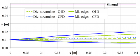
Figure 2 shows the dividing streamline and shear layer edges for case 1. The edges for CFD results are calculated by the same method as explained for the Q1D (section 3).
Although the agreement appear to be quite satisfactory, it is important to point out that the illustrated trends represent a rough approximation of the real shear layer. In particular, the assumption of a linear velocity profile causes an underestimation of the actual shear layer thickness. A better estimation can be obtained by means of different thickness definitions or by releasing the linear approximation in favor of a more appropriate hyperbolic tangent velocity profile.
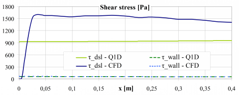
Figure 3 from a to c show the results in terms of mach, velocity, temperature and density variations. The oscillations of the CFD results for the primary streams are due to the presence of subsequent trains of expansions and shocks of the supersonic primary stream. These come from small residual pressure gradients due to an imperfect matching of the pressure conditions. Although in principles these could be reduced, in practice it is impossible to perfectly match the pressure conditions as gradients are produced internally by the strong shear exchange. This is also the cause of the turbulence production which allows for intense mixing between the two streams. Figure 3c shows that the density is approximately constant and equal for the two streams, partly validating the hypothesis made in section 3 for the calculations of the shape profiles. The greatest departure between the two methods is seen for the results related to the primary stream Mach number, where the data for Q1D model are quite above those from CFD results. The reason for this error becomes clear by looking at figure 4, which shows the variation of the shear stress at wall and on the dividing streamline.
Table 2. Comparison of theoretical and numerical final results for the various cases
|
|
Case 1 |
Case 2 |
Case 3 |
Case 4 |
|||||||||
|
Variable |
Unit |
Q1D |
CFD |
%Err. |
Q1D |
CFD |
%Err. |
Q1D |
CFD |
%Err. |
Q1D |
CFD |
%Err. |
|
m1 |
kg/s |
0.168 |
0.168 |
0.4 |
0.184 |
0.184 |
0.3 |
0.207 |
0.206 |
0.3 |
0.234 |
0.234 |
0.3 |
|
m2 |
kg/s |
1.395 |
1.359 |
2.7 |
1.318 |
1.283 |
2.8 |
1.135 |
1.068 |
6.3 |
0.851 |
0.475 |
79.1 |
|
ER |
- |
8.3 |
8.1 |
2.3 |
7.2 |
7.0 |
2.4 |
5.5 |
5.2 |
5.9 |
3.6 |
2.0 |
78.6 |
Figure 2. Mixing layer edges and dividing streamline for case 1
Figure 3. Mach (a), Temperature (b) and density profiles (c) along the mixing chamber for case 1
Figure 4. Shear stress on the dividing streamline (left axis) and at wall (right axis) for case 1
The Q1D model underestimates the shear stress by around 30% with respect to CFD data. This causes a lower momentum transport from the primary to the secondary stream. Moreover, being the primary mass flow rate much lower than that of secondary flow, this error impacts almost exclusively the primary velocity. Conversely, results for the shear stress at wall show an excellent agreement with CFD results. This is important in that it demonstrates that the main source of error comes almost exclusively from the modeling of the momentum exchange along the dividing streamline. In particular, the lower shear stress predicted by the Q1D model is most likely due to excessive turbulence suppression by the compressibility correction, eq. 5. Although this could be calibrated to better match the numerical data, nevertheless, in much the same way as for the shear layer spreading rate, the CFD value of the shear stress is calculated by means of ad-hoc corrections. Therefore, a more reliable comparison and calibration should be carried out by comparing the Q1D results directly with experimental data.
Finally, figure 4 shows that the numerical shear stress at the entrance of the mixing chamber is almost zero. This is due to the presence of a developing region of the mixing layer. After a distance of around 5 mm the shear layer turbulence has grown to its fully turbulent state and viscous effects becomes negligible. This phenomenon cannot be captured by the Q1D as the correlation for the shear stress, eq. 6, is valid only in the region of fully developed turbulent mixing layer
In order to optimize the mixing inside a supersonic ejector, the momentum exchange must be maximized while reducing irreversibilities. Sources of losses inside the mixing chamber include heat exchange between the two streams, supersonic shocks, friction and heat losses at wall, turbulence production and dissipation. As already discussed in previous sections, the first two sources can be minimized by matching the inlet static states of the two streams. As for friction losses, benefits can be achieved by reducing the wall roughness and by decreasing the mixing chamber length. Short mixing chambers can be obtained by increasing the mixing effectiveness, i.e., by increasing the mixing layer spreading rate and shear stress.
There have been a number of attempts to increase the mixing rate by methods of mixing enhancement such as vortex generators, tripped boundary layers, swirlers and cross blowing [7]. However, in many cases it is unclear whether the benefits are worth the additional pressure losses.
Looking at eq. 4, larger values of spreading rate can be achieved by:
In case of constant pressure mixing of a single gas, increasing the density ratio would translate in larger temperature difference, thus resulting in heat transfer losses. As for the velocity ratio, the speed of the secondary stream should always be the least possible. This can be achieved by controlling the pressure along the mixing chamber, which must be as close as possible to the secondary stream total pressure (this also leads to lower recompression rate in the ejector diffuser). The Q1D model could be easily exploited for this purpose as it permits quick calculations of many different mixing chamber profiles.
The problem becomes more complicated for the primary stream velocity. In the simplified case of constant pressure and temperature mixing of a single gas, the speed of sound of the two streams are approximately the same (this is true just at the beginning of the mixing region while at farther distances temperatures will change due to the slow down or acceleration of the streams, see figure 3b). In this case, the convective Mach number becomes:
$M_{c}=\frac{\Delta U_{\infty}}{a_{\infty 1}+a_{\infty 2}} \approx \frac{M_{\infty 1}-M_{\infty 2}}{2}$(34)
If we further assume that secondary stream velocity is negligible with respect to primary speed, the shear layer spreading rate, eq. 4, simplifies to:
$\delta_{\omega}^{\prime}=0.085 \cdot\left[0.25+0.75 e^{-3 M_{\infty 1}^{2}}\right]$(35)
which is a monotonically decreasing function of the primary stream Mach number. Therefore, increasing the primary stream speed necessarily causes a reduction of the mixing rate. As the nozzle exit pressure of the ejector must match that of the secondary stream, a reduction of the primary stream Mach number can be obtained by only two methods: increasing the secondary stream pressure or decreasing the inlet primary total pressure. As mentioned above, the first method should always be pursued. However, the secondary pressure can be raised only up to the value of inlet total pressure, thus limiting the extent of possible benefits.
There are limits also to the reduction of inlet primary total pressure. Supersonic ejectors for heat powered chillers serve the purpose of transferring mechanical energy between the motive and the refrigeration cycle. When the primary total pressure is lowered, the amount of mechanical energy entering the ejector decreases and the refrigeration load is abated. This can be avoided by increasing the primary mass flow rate. However, this leads to a reduction of contact surface per unit volume of the primary flow that again reduces the mixing effectiveness inside the mixing chamber.
One way to overcome these limitations is represented by the optimization of the shear surfaces between primary and secondary streams. As seen before, increasing the length of the mixing chamber is not a valuable solution as friction losses grow. In addition, the increase in contact surface is obtained in far regions where gradients and entrainment rate are lower. Therefore, more advanced solutions could derive from new design configurations of the primary nozzle, e.g., annular primary nozzle [19], petal nozzles [20] and multiple nozzles [21]. This last solution basically consists in a partition of the primary mass flow rate that is redirected through many smaller nozzles, whose sizes and positions must be carefully designed.
In order to demonstrate these concepts, a simple optimization was tried for a planar mixing chamber of 0.4x0.4x0.2m length, height and width respectively. By keeping the boundary conditions fixed, the primary stream was allowed to flow through an increasing number of primary nozzles (1, 2 and 4), uniformly spaced along the vertical direction. The boundary conditions are the same as those presented in table 1, except that the outlet pressure is 60 000 Pa.
Table 3 shows the global results of the optimization. The entrained secondary flow increases by 11.9% passing from the single nozzle configuration to the 2 nozzles design. The growth of secondary flow is even larger when splitting the primary stream into 4 nozzles, with 28% difference with respect to the original configuration. Passing from the single nozzle configuration to that with 4 nozzles, the Mach number of the primary stream increases while that of secondary flow decreases. This is a clear indication of greater mixing.
Table 3. Global results of the planar mixing chamber optimization
|
Variable |
Unit |
1 nozzle |
2 nozzles |
4 nozzles |
|
m1 |
Kg/s |
8.24 |
8.24 |
8.24 |
|
m2 |
Kg/s |
7.86 |
8.80 |
10.07 |
|
ER |
- |
0.95 |
1.07 |
1.22 |
|
P – inlet |
kPa |
56,7 |
53,2 |
44,7 |
|
P – outlet |
kPa |
60 |
60 |
60 |
|
Ma1 – outlet |
- |
2.5 |
2.4 |
2.2 |
|
Ma2 – outlet |
- |
0.47 |
0.53 |
0.63 |
|
δω – outlet |
m |
1x0.0132 |
2x0.0128 |
4x0.0121 |
The main reason for these improvements is to be found in the significant increase in contact surface between the two streams. Although the shear layer of the single nozzle is greater than those of other configurations, the splitting of the primary stream increase the number of mixing layers, i.e., the total shear surface inside the mixing chamber. Figure 5 clearly illustrates this concept by showing all together the shear region for the 3 cases.
The calculation presented above is only one example among many other possible applications. Indeed, by means of a simple mixing model like that presented here, a constructal optimization may be performed in order to find the best design in terms of sizes and number of primary nozzles, distance between the nozzles and from the external surface, length of the mixing chamber. In practice, the use of the Q1D approximation allows regarding the ejector as an equivalent “momentum exchanger” between two coflowing streams. Consequently, many of the Constructal design concepts that were developed for the optimization of heat exchangers [22] may be applied.
Figure 5. Half section of the planar mixing chamber; colored regions represent the shear layers
An analytical scheme that describes the turbulent mixing zone within an ejector was presented. The model is able to compute all flow properties inside an axisymmetric or planar mixing chamber with either constant or variable cross section. The amount of entrained flow, the work and heat exchange, pressure losses and mixing efficiency are computed as a function of the system geometry and without use of any arbitrary parameter. Consequently, this model is particularly suited for a thermodynamic optimization of the ejector system.
The model was validated by comparison with CFD results for various operating conditions. Results generally showed good agreement in all parameters, with increasing errors as pressure gradient increases. In particular, discrepancy between numerical and theoretical Entrainment Ratio was generally well below 10%.
One of the main problems in the optimization of a supersonic ejector is the decrease of mixing effectiveness with increasing primary stream Mach number. A way to work around this problem is to enlarge and optimize the contact surfaces between primary and secondary stream.
A preliminary study was performed in this direction. Results demonstrated that splitting the primary mass flow into several smaller nozzles (ceteris paribus), notably increases the entrainment of the secondary flow.
This result leads the way to new design configurations that may be optimized by means of a constructal approach. The Q1D model presented here is particularly suitable to this aim, in that it envisions the ejector as an equivalent “momentum exchanger”. Consequently, many of the Constructal design concepts that were developed for the optimization of heat exchangers may be applied.
We wish to thank Professor Papamoschou for his willingness and valuable help.
1. ESDU Ejectors and jet pumps, Data item 86030, ESDU International Ltd, London, UK, 1986.
2. Papamoschou, D., “Model for entropy production and pressure variation in confined turbulent mixing,” AIAA journal, 31(9), 1643-1650, 1993. DOI: 10.2514/3.11826.
3. Papamoschou, D., “Analysis of partially mixed supersonic ejector,” Journal of propulsion and power, 12(4), 736-741, 1996. DOI: 10.2514/3.24096.
4. Brown, G. L., Roshko, A., “On density effects and large structure in turbulent mixing layers,” Journal of Fluid Mechanics, 64(4), 775–816, 1974. DOI: 10.1017/S002211207400190X.
5. Bejan, A., Entropy Generation through Heat and Fluid Flow, John Wiley and Sons, inc., 1982.
6. Holmes, P., Lumley, J.L., Berkooz, G., Rowley, C.W., Turbulence, Coherent Structures, Dynamical Systems and Symmetry, Cambridge University Press, 2012.
7. Smits, A.J., Dussauge, J., Turbulent Shear Layers in Supersonic Flow, Second Edition, Springer Science+Business Media Inc., 2006.
8. Gatsky, T.B., Bonnet, J.P., Compressibility, Turbulence and High Speed Flow, 2nd edition, Academic Press, Oxford, UK, 2013.
9. Ikawa, H., “Turbulent mixing layer experiments in supersonic flow,” Ph.D. Thesis, California Institute of Technology, Pasadena, CA, 1973.
10. Papamoschou, D., Roshko, A., “The compressible turbulent shear layer: An experimental study,” Journal of Fluid Mechanics, 197, 453–477, 1988. DOI: 10.1017/S0022112088003325.
11. Wygnanski, I., Fiedler, H.E., “The two-dimensional mixing region,” Journal of Fluid Mechanics, 41, 327–362, 1970. DOI: 10.1017/S0022112070000630.
12. Townsend, A.A., The Structure of Turbulent Shear Flow, 2nd edition, Cambridge University Press, 1976.
13. Mazzelli, F., Milazzo, A., “Performance analysis of a supersonic ejector cycle working with R245fa,” International Journal of Refrigeration, 49(0), 79-92, 2015. DOI: 10.1016/j.ijrefrig.2014.09.020.
14. Schlichting, H., Boundary-Layer Theory, 7th edition, McGraw-Hill, 1979.
15. Hickman, K.E., Hill, P.G., Gilbert, G.B., “Analysis and testing of compressible flow ejectors with variable area mixing tubes,” Journal of Basic Engineering, Trans. ASME, 407-416, 1972. DOI: 10.1115/1.3425436.
16. Rajaratnam, N., Turbulent Jets, Elsevier scientific publishing company, 1976.
17. Barone, M.F., Oberkampf, W.L., Blottner, F.G., “Validation case study: Prediction of compressible turbulent mixing layer growth rate,” AIAA Journal, 44(7), 1488–1497, 2006. DOI: 10.2514/1.19919.
18. Wilcox, D.C., “Dilatation-dissipation corrections for advanced turbulence models,” AIAA Journal, 30(11), 2639-2646, 1992.
19. Kim, S., Jin, J., Kwon, S., “Experimental investigation of an annular injection supersonic ejector,” AIAA Journal, 44(8), 1905–1908, 2006. DOI: 10.2514/1.16783.
20. Srikrishnan, A.R., Kurian, J., Sriramulu, V., “Experimental study on mixing enhancement by petal nozzle in supersonic flow,” Journal of Propulsion and Power, 12(1), 165-169, 1996. DOI: 10.2514/3.24006.
21. Chandrasekhara, M.S., Krothapalli, A., Baganoff, D., “Performance characteristics of an underexpanded multiple jet ejector,” Journal of Propulsion and Power, 7(3), 462-464, 1991. DOI: 10.2514/3.23348.
22. Bejan, A., Lorente, S., Design with Constructal Theory, John Wiley & Sons, Inc., Hoboken, New Jersey, 2008.