OPEN ACCESS
Here we show how a heat generating domain can be gained self-cooling capability with embedded cooling channels and with and without high-conductivity fins. The volume of the heat generating domain is fixed, so is the overall volume of the cooling channels and high-conductivity inserts. Even though the coolant volume decreases with embedded high-conductivity fins, the peak temperature also decreases with high-conductivity inserts. The peak temperature is affected by the location, shape and complexity of the fins and the volume fraction. This paper documents how these degrees of freedoms should be changed in order to minimize peak temperature. This paper also discusses how the volume fraction affects each fin shape in order to minimize the peak temperature. This paper uncovers that the fins should be distributed non-equidistantly, and that high-conductivity material should be inserted as fins (bulks of high-conductivity materials) rather than uniform distribution in the domain. This paper concludes that the overall thermal conductance of a heat generating domain can be maximized by freely morphing the shape of the high-conductivity material. The optimal design exists for given conditions and assumptions, and this design should be morphed when conditions and assumptions change. This conclusion is in accord with the constructal law. Each optimal design for given conditions and assumptions is the constructal design.
Constructal, Self-cooling, High-conductivity, Conduction, Inverted fins.
The trend of miniaturization in advanced technologies require compactness with great volumetric heating rates. For instance, heat generation rate per unit volume in current electronic chips is equivalent to the one in nuclear reactors [1]. Therefore, cooling became a challenge due to miniaturization. The heat transfer surface areas of miniature designs is not enough in order to cool themselves with natural convection and forced convection when the coolant fluid is air. Therefore, forced convection with distinct coolants such as water, oil and nano-fluids, and heat transfer enhancement with extended surfaces are focused in the current literature [2-10]. In addition, different optimization parameters such as spacing in between electronic boards and non-uniform chip distribution are also discussed in the literature [11-16]. However, coolant fluid always interact with solid domains in convection in order to cool mechanical systems. When the thermal resistance of the convective domain is so small in comparison with the thermal resistance of the conductive domain, the rate of the heat transfer is dominated by the conductive thermal resistance. In the heat transfer field, the conductive resistances are neglected as a tradition because the thermal resistances of solids (such as the resistance of a copper pipe in a heat exchanger) is smaller than convective resistances. However, as compactness increases the effect of the conductive resistances on the overall thermal resistance increases. Therefore, increasing the convective heat transfer coefficient after a ceiling value does not change the order of the overall heat transfer rate while the conductive resistances kept the same.
“Constructal law” shows how the shape should be morphed freely in order to minimize resistances in a flow system (flow of heat, fluid and/or stress) [15-18]. Constructal law is used in distinct fields such as engineering, biology, geology and physics [15-24]. In addition, this law shows the connection between these fields by uncovering how the designs evolve in time in order to minimize resistances, and how the designs in distinct fields look alike because their designs are governed by the same objective, i.e. design of river-deltas, human lung, Eiffel tower, lightning bolts and trees have the same objective: minimization of resistances to the flow of fluid, heat and stress [18, 25].
Almogbel and Bejan [26] showed that embedding high-conductivity materials in heat generating domains increases the overall thermal conductance of the domains. In addition, literature also shows how thermal conductance of a domain can be maximized with distinct high-conductivity inserts: tree-shaped (T- and Y-shaped) and 2- and 3-dimensional with and without non-uniform heating [1, 26-32]. In the literature, tree-shaped high-conductivity materials are embedded in heat generating domains, and their stem are assumed to be a heat sink at prescribed temperature. However, constant stem temperature would be impossible to implement when the heat generating domains are elemental domains, i.e. a part of a system which consists of many number of identical elemental domains. Therefore, the literature lacks of commenting on how to carry heat from the stem of the high-conductivity insert to a coolant fluid. This paper discusses how to use high-conductivity inserts in palpable devices with realistic boundary conditions.
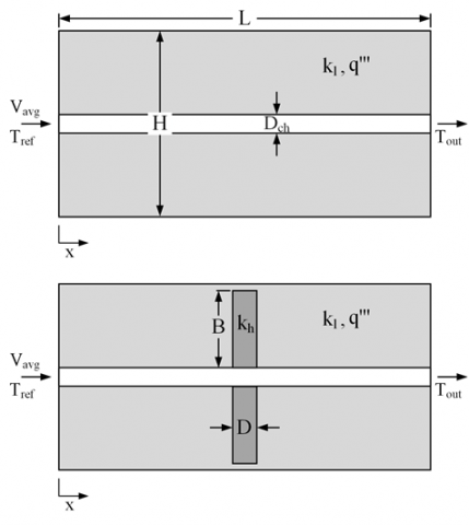
Consider a rectangular domain with width of L and height of H, Fig. 1. This domain is heated volumetrically and a channel of diameter Dch is embedded along the width of the domain in which coolant fluid flows, Fig. 1 (top). Coolant fluid enters with Vavg average velocity and Tref inlet temperature, and it leaves the channel with Tout outlet temperature. These temperatures are the mean of temperature profile in the vertical direction of the channel. The heat conductivity of the solid domain is $\mathrm{k}_{1}$. In addition, high-conductivity fins of thermal conductivity $\mathrm{k}_{\mathrm{h}}$ embedded in the solid heat generating domain as shown in Fig. 1 (bottom). The summation of the cooling channel area and high-conductivity inserts area is fixed, so is the heat generating solid area. Their ratio defined as $\phi$ volume fraction. The stems of the high-conductivity inserts are attached on the interface of the coolant channel. In addition, the boundary condition of the outside boundaries is symmetry boundary condition ($\partial \mathrm{T} / \partial \mathrm{n}=0$) because the rectangular domain discussed in this paper is an elemental area of a greater domain consists of multiple and identical elemental domains.
Figure 1. Heat generating domain cooled by embedded channel in which coolant fluid flow without high conductivity inserts (top) and with high conductivity inserts (bottom)
The fluid flow is governed by the conservation of mass and momentum equations for incompressible steady flow with constant properties and single phase in a two-dimensional domain
$\frac{\partial \mathrm{u}}{\partial \mathrm{x}}+\frac{\partial \mathrm{v}}{\partial \mathrm{y}}=0$(1)
$\mathrm{u} \frac{\partial \mathrm{u}}{\partial \mathrm{x}}+\mathrm{v} \frac{\partial \mathrm{u}}{\partial \mathrm{y}}=-\frac{1}{\rho} \frac{\partial \mathrm{P}}{\partial \mathrm{x}}+v \nabla^{2} \mathrm{u}$(2)
$\mathrm{u} \frac{\partial \mathrm{v}}{\partial \mathrm{x}}+\mathrm{v} \frac{\partial \mathrm{v}}{\partial \mathrm{y}}=-\frac{1}{\rho} \frac{\partial \mathrm{P}}{\partial \mathrm{y}}+v \nabla^{2} \mathrm{v}$(3)
Here x and y are the longitudinal and vertical spatial coordinates, u and v are the velocity components corresponding to these coordinates, and P, ν and ρ are the pressure, kinematic viscosity and fluid density.
The temperature distribution inside the cooling channel is governed by the energy equation for fluid domain
$\rho \mathrm{c}_{\mathrm{P}}\left(\mathrm{u} \frac{\partial \mathrm{T}}{\partial \mathrm{x}}+\mathrm{v} \frac{\partial \mathrm{T}}{\partial \mathrm{y}}\right)=\mathrm{k}_{\mathrm{f}} \nabla^{2} \mathrm{T}$(4)
where cp, T and kf are the specific heat at constant pressure of the fluid, temperature and fluid thermal conductivity, respectively.
The governing equations for the low-conductivity and high-conductivity solid domains are,
$\mathrm{k}_{1} \nabla^{2} \mathrm{T}=\mathrm{q}^{\prime \prime \prime}$(5)
$\mathrm{k}_{\mathrm{h}} \nabla^{2} \mathrm{T}=0$(6)
where $\mathrm{q}^{\prime \prime \prime}$ is the volumetric heat rate and $\nabla^{2}=\partial^{2} / \partial \mathrm{x}^{2}+\partial^{2} / \partial \mathrm{y}^{2}$. The continuity of heat flux between the high-conductivity and low-conductivity solids and fluid interfaces requires
$\mathrm{k}_{1} \frac{\partial \mathrm{T}}{\partial \mathrm{n}}=\mathrm{k}_{\mathrm{h}} \frac{\partial \mathrm{T}}{\partial \mathrm{n}}, \mathrm{k}_{1} \frac{\partial \mathrm{T}}{\partial \mathrm{n}}=\mathrm{k}_{\mathrm{f}} \frac{\partial \mathrm{T}}{\partial \mathrm{n}}, \mathrm{k}_{\mathrm{h}} \frac{\partial \mathrm{T}}{\partial \mathrm{n}}=\mathrm{k}_{\mathrm{f}} \frac{\partial \mathrm{T}}{\partial \mathrm{n}}$(7)
where n is the vector normal to the fluid-solid or high-conductivity solid-low-conductivity solid interface.
Equations (1) – (3) are nondimensionalized by using L as the length scale, and constructing dimensionless velocities in the form of Reynolds numbers
$(\tilde{\mathrm{x}}, \tilde{\mathrm{y}}, \tilde{\mathrm{z}}, \tilde{\mathrm{n}})=(\mathrm{x}, \mathrm{y}, \mathrm{z}, \mathrm{n}) / \mathrm{L}$
$\tilde{\mathrm{u}}=\mathrm{uL} / v$
$\tilde{\mathrm{v}}=\mathrm{vL} / v$
$\tilde{\mathrm{w}}=\mathrm{wL} / v$(8)
The dimensionless pressure difference is defined as Bejan number [33-34]
$\tilde{\mathrm{P}}=\frac{\left(\mathrm{P}-\mathrm{P}_{\mathrm{out}}\right) \mathrm{L}^{2}}{\mu \alpha}$(9)
where P, Pout, μ and $\alpha$ are the local pressure, outlet pressure, dynamic viscosity and thermal diffusivity of the fluid ($\alpha=k_{f} / \rho c_{p}$). The dimensionless temperature and continuity of the heat flux on solid-fluid and high-conductivity solid-low-conductivity solid interfaces are indicated by
$\tilde{\mathrm{T}}=\frac{\left(\mathrm{T}-\mathrm{T}_{\mathrm{ref}}\right) \mathrm{k}_{\mathrm{f}}}{\mathrm{q}^{\mathrm{w}} \mathrm{L}^{2}}$(10)
\(\text{5\tilde{k}}{{\left. \frac{\partial \text{\tilde{T}}}{\partial \text{\tilde{n}}} \right|}_{\text{h}}}\text{ }={{\left. \frac{\partial \text{\tilde{T}}}{\partial \text{\tilde{n}}} \right|}_{\text{l}}}\), \(\text{\tilde{k}}{{\left. \frac{\partial \text{\tilde{T}}}{\partial \text{\tilde{n}}} \right|}_{\text{l}}}\text{ }={{\left. \frac{\partial \text{\tilde{T}}}{\partial \text{\tilde{n}}} \right|}_{\text{f}}}\), \(\text{100\tilde{k}}{{\left. \frac{\partial \text{\tilde{T}}}{\partial \text{\tilde{n}}} \right|}_{\text{h}}}\text{ }={{\left. \frac{\partial \text{\tilde{T}}}{\partial \text{\tilde{n}}} \right|}_{\text{f}}}\) (11)
where Tref is the fluid inlet temperature and $\tilde{\mathrm{k}}=\mathrm{k}_{1} / \mathrm{k}_{\mathrm{f}}$.
The dimensionless mass conservation and momentum equations are
$\frac{\partial \tilde{\mathrm{u}}}{\partial \tilde{\mathrm{x}}}+\frac{\partial \tilde{\mathrm{v}}}{\partial \tilde{\mathrm{y}}}=0$(12)
$\tilde{\mathrm{u}} \frac{\partial \tilde{\mathrm{u}}}{\partial \tilde{\mathrm{x}}}+\tilde{\mathrm{v}} \frac{\partial \tilde{\mathrm{u}}}{\partial \tilde{\mathrm{y}}}=-\frac{1}{\mathrm{Pr}} \frac{\partial \tilde{\mathrm{P}}}{\partial \tilde{\mathrm{x}}}+\tilde{\nabla}^{2} \tilde{\mathrm{u}}$(13)
$\tilde{\mathrm{u}} \frac{\partial \tilde{\mathrm{v}}}{\partial \tilde{\mathrm{x}}}+\tilde{\mathrm{v}} \frac{\partial \tilde{\mathrm{v}}}{\partial \tilde{\mathrm{y}}}=-\frac{1}{\mathrm{Pr}} \frac{\partial \tilde{\mathrm{P}}}{\partial \tilde{\mathrm{y}}}+\tilde{\nabla}^{2} \tilde{\mathrm{v}}$(14)
where Pr is Prandtl number and $\tilde{\nabla}^{2}=\partial^{2} / \partial \tilde{\mathbf{x}}^{2}+\partial^{2} / \partial \tilde{y}^{2}$. The dimensionless energy equation is
$\operatorname{Pr}\left(\tilde{\mathrm{u}} \frac{\partial \tilde{\mathrm{T}}}{\partial \tilde{\mathrm{x}}}+\tilde{\mathrm{v}} \frac{\partial \tilde{\mathrm{T}}}{\partial \tilde{\mathrm{y}}}+\tilde{\mathrm{w}} \frac{\partial \tilde{\mathrm{T}}}{\partial \tilde{\mathrm{z}}}\right)=\nabla^{2} \tilde{\mathrm{T}}$(15)
The dimensionless governing equations of Eqs. (5) and (6) are
$\tilde{\mathrm{k}} \tilde{\mathrm{V}}^{2} \tilde{\mathrm{T}}=1$(16)
$\tilde{\nabla}^{2} \tilde{\mathrm{T}}=0$(17)
Consider the two-dimensional domain shown in Fig. 1(bottom) along which coolant fluid flows at Vavg inlet velocity and with reference temperature (Tref). Volumetric heating rate on the domain of thermal conductivity kl is $\mathrm{q}^{\prime \prime \prime}$. High-conductivity material with height of B and thickness of D is embedded on the solid domain as shown in Fig. 1 (bottom). Dimensionless inlet average velocity is 2000, Prandtl number is 6, H/L = 1, D/B = 0.15 and $\phi=0.1$.
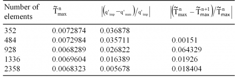
The dimensionless conservation of mass, momentum and energy equations were solved by using a finite element software [35]. The grid was non-uniform in both directions. Boundary layer meshes are also used at the interfaces in order to minimize the numerical errors due to variation in the temperature gradients. The mesh size was determined by increasing the number of the mesh elements until the criterion $\left|\left(\tilde{\mathrm{T}}_{\max }^{\mathrm{n}}-\tilde{T}_{\max }^{n+1}\right) / \tilde{T}_{\max }^{n}\right|<2 \times 10^{-2}$ was satisfied. $\tilde{\mathrm{T}}_{\max }^{\mathrm{n}} \quad$ and $\quad \tilde{T}_{\mathrm{max}}^{n+1}$ represent the maximum dimensionless temperature by using the current mesh and the refined mesh, respectively. Table 1 illustrates that mesh independency was achieved with 2358 number of mesh elements for the design shown in Figure 1 (bottom).
In addition, the overall heat transfer rate on the stem surface of the high-conductivity insert ($\mathrm{q}_{\mathrm{num}}^{\prime}$) is compared with the heat transfer rate calculated from the heat generation rate ($\mathbf{q}_{\text { imp }}^{\prime}$) as shown in Table 1. The error in between the generated heat and the transferred heat was found as 0.5% for the selected mesh size. This shows that the 1st law of thermodynamics is also satisfied. The numerical results obtained by using the current method have been compared with the numerical results of Almogbel and Bejan [26] for the validation of the numerical method. The dimensionless governing equations of Ref. [26] was solved with the given geometry and boundary conditions when $\varphi=0.1, \mathrm{H} / L=1$ and $\mathrm{D} / B=0.15$. Table 2 shows that the results of the current numerical method agrees with the results of Ref. [26].
Table 1. Numerical tests showing that the result of the simulations is independent of the mesh size
Table 2. Comparison of the results of the current numerical study+ and Ref. [26]*
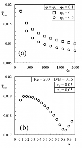
Consider the high-conductivity inserts of thermal conductivity kh and length scales of D and B embedded in a heat generating domain. This domain is cooled by a coolant fluid which flows along the domain as shown in Fig. 1 (bottom). The heat generating domain is an elemental part of a greater domain. Figure 2a shows that how the peak temperature is affected by the volume fraction (coolant volume/heat generating domain volume) when the elemental domain is solely cooled by convection via flowing coolant along the channel with Re = 2000. Peak temperature decreases as the volume fraction increases. However, it should be in mind that as volume fraction increases the heat generating domain volume also decreases, i.e. the rate of total heat generation decreases.
Figure 2b shows how the location of the high-conductivity insert affects peak temperature when both $\varphi_{\mathrm{f}}$ (coolant fluid volume/heat generating domain volume) and $\varphi_{\mathrm{s}}$ are fixed at 0.05. The summation of the coolant volume and high-conductivity material volume over the heat generating domain is $\varphi=\varphi_{\mathrm{s}}+\varphi_{\mathrm{f}}=0.1$. Comparison of Fig. 2a with $\varphi=0.1$ and Fig. 2b shows that embedding high-conductivity inserts decreases the peak temperature from 0.009 to 0.0084 – 0.0064 range for a specific x location of the high-conductivity insert. This comparison shows that embedding high-conductivity inserts increases the overall thermal conductance of a heat generating domain. Therefore, embedding high-conductivity inserts with convective cooling provides greater cooling performance in comparison with solely convective cooling. In addition, Figure 2c shows how D/B ratio affects the peak temperature. It is the smallest with D/B = 0.11 when Re = 2000, x = 0.6 and $\varphi=0.1$.
Figure 2. (a) The effect of coolant volume fraction on maximum temperature without high-conductivity inserts. (b) The effect of the location of the high-conductivity inserts on maximum temperature. (c) The effect of the shape of the inserts on maximum temperature
Figure 3a shows how Reynolds number (i.e. dimensionless average inlet velocity) affects the peak temperature with and without high-conductivity inserts as shown in Fig. 1. The effect of inserting high-conductivity inserts is negligibly small in comparison with the peak temperature when Re = 200 because the generated heat is greater than the heat capacitance of the coolant fluid. Therefore, peak temperature decreases with high-conductivity inserts when Re > 200. In addition, the return of increasing Re number decreases as Re increases. Figure 3b shows that the effect of location of the high-conductivity insert along the x direction when Re = 200. The trend of Figure 3b is similar to the trend of Figure 2b, however, the x location which provides the smallest peak temperature is moved from x = 0.6 to x = 0.85 as Re decreases from 2000 to 200.
Figure 3. (a) The effect of Re number on peak temperature with and without high-conductivity inserts. (b) The effect of the location of the high-conductivity inserts on peak temperature with Re = 200.
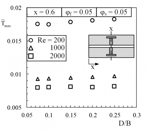
Figure 4 shows the effect of D/B ratio on the peak temperature with tree-shaped high-conductivity inserts when Re = 200, 1000 and 2000. The tree-shaped insert is located at x = 0.6 which provides the smallest peak temperature when Re = 2000 as shown in Fig. 2b. Figure 4 is also in accord with Fig. 3a, i.e. the peak temperature decreases as Re number increases and this increase diminishes as Re number increases. Figure 4 shows that peak temperature is the smallest with D/B = 0.1, 0.075 and 0.075 for Re = 200, 1000 and 2000, respectively. In addition, the peak temperature decreases as inserting T-shaped high-conductivity insert instead of a rectangular insert as shown in Fig. 1. However, the decrease in the peak temperature is so small by embedding T-shaped insert instead of rectangular one in comparison with the order of the peak temperature, i.e. peak temperature decreases 0.03% by morphing the insert to a T-shaped design.
Figure 4. The effect of D/B ratio of a T-shaped tree design with Re = 200, 1000 and 2000
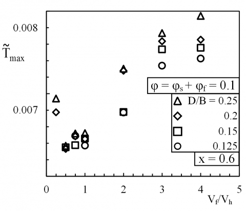
Figure 5 shows how $\mathrm{V}_{\mathrm{f}} / \mathrm{V}_{\mathrm{h}}$(volume of the coolant fluid/volume of the high-conductivity material) affects $\tilde{\mathbf{T}}_{\max }$ as D/B varies for the design shown in Fig. 1(bottom). As $\mathrm{V}_{\mathrm{f}} / \mathrm{V}_{\mathrm{h}}$ increases from 0.25 to 1 the effect of varying D/B on $\tilde{\mathbf{T}}_{\max }$ becomes 2% maximum. Effect of varying D/B ratio on $\tilde{\mathbf{T}}_{\max }$ becomes up to 7% as $\mathrm{V}_{\mathrm{f}} / \mathrm{V}_{\mathrm{h}}$ becomes 4. In addition, as $\mathrm{V}_{\mathrm{f}} / \mathrm{V}_{\mathrm{h}}$ increases from 1 to 4 $\tilde{\mathbf{T}}_{\max }$ is the minimum with D/B =0.125. Note that for $\mathrm{V}_{\mathrm{f}} / \mathrm{V}_{\mathrm{h}}=0.25$, D/B value cannot be taken less than 0.2 because high-conductivity inserts penetrate the walls of the heat generating domain when D/B < 0.2. In addition, $\tilde{\mathbf{T}}_{\max }$ is minimum when $\mathrm{V}_{\mathrm{f}} / \mathrm{V}_{\mathrm{h}}=0.5$, i.e., high-conductivity material volume is two times the coolant volume, Fig. 5.
Figure 5. The effect of the ratio of coolant volume to high-conductivity material volume on maximum temperature for D/B = 0.125, 0.15, 0.2 and 0.25
This paper shows that the peak temperature of a heat generating domain which is cooled with embedded cooling channels can be decreased with inserting high-conductivity material. The volume of the heat generating domain is fixed, so is the summation of the cooling channels and high-conductivity material volumes. Embedding high-conductivity inserts increases the overall thermal conductance of the heat generating domain even though coolant volume reduces due to fixed volume constraint. This paper also shows that high-conductivity material should be located a little bit further from the middle and closer to the coolant outlet, i.e. namely x = 0.6 when Re = 2000. This paper also shows the optimal fin locations which corresponds the smallest peak temperature is affected by the average inlet velocity. The optimal location moves closer to the outlet as Re number decreases. These findings are essential because the current literature does not cover the effect of location of the high-conductivity inserts and the effect of convection on the thermal conductance of a heat generating domain in which high-conductivity material is embedded. In addition, the effect of shape and volume fraction on the peak temperature is also documented.
Furthermore, distributing high-conductivity material homogenously into the heat generating domain does not decrease the peak temperature as embedding inserts with the optimized shapes and locations documented in this paper. The high-conductivity material should be inserted such that the overall thermal conductance of the heat generating domain becomes the greatest, i.e. as the volume fraction and boundary conditions change the shape and locations of the fins should be changed.
This work was supported by the Scientific and Technological Research Council of Turkey (TUBITAK) under grant number 114M592.
1. Cetkin, E., “Inverted fins for cooling of a non-uniformly heated domain,” J. Thermal Engineering, 1, pp. 1−9, 2015.
2. Bejan, A. and Ledezma, G.A., “Thermodynamic optimization of cooling techniques for electronic packages,” Int. J. Heat Mass Transfer, 39(6), pp. 1213−1221, 1996. DOI: 10.1016/0017-9310(95)00196-4.
3. Said, S.A.M., “Investigation of natural convection in convergent vertical channels,” Int. J. Energy Res., 20, pp. 559−567, 1996. DOI: 10.1002/(SICI)1099-114X(199607)20:7<559::AID-ER115>3.0.CO;2-J.
4. Jang, D., Yook, S.J. and Lee, K.S., “Optimum design of a radial heat sink with a fin-height profile for high-power led lighting applications”. Appl. Energy, 116, pp. 260−268, 2014. DOI: 10.1016/j.apenergy.2013.11.063.
5. Ho, T., Mao, S.S. and Greif, R., “Improving efficiency of high-concentrator photovoltaics by cooling with two-phase forced convection” Int. J. Energy Res., 34, pp. 1257−1271, 2010. DOI: 10.1002/er.1670.
6. Kakac, S., Pramuanjaroenkij, A., “Review of convective heat transfer enhancement with nanofluids,” Int. J. Heat Mass Transfer, 52, pp. 3187−3196, 2009. DOI: 10.1016/j.ijheatmasstransfer.2009.02.006.
7. Eastman, J.A., Choi, S.U.S., Li, S., Yu, W. and Thompson, L.J., “Anomalously increased effective thermal conductivities of ethylene glycol-based nanofluids containing copper nanoparticles,” Appl. Phys. Lett., 78, pp. 718−720, 2001. DOI: 10.1063/1.1341218.
8. Lorenzini, G., Correa, R.L., dos Santos, E.D. and Rocha, L.A.O., “Constructal design of complex assembly of fins,” J. Heat Transfer, 133(8), 081902, 2011. DOI: 10.1115/1.4003710.
9. Bejan, A. and Morega, A.M., “Optimal arrays of pin fins and plate fins in laminar forced-convection,” J. Heat Transfer, 115(1), pp. 75−81, 1993. DOI: 10.1115/1.2910672.
10. Lorenzini, G. and Moretti, S., “Bejan’s constructal theory analysis of gas-liquid cooled finned modules,” J. Heat Transfer, 133(7), 071801, 2011. DOI: 10.1115/1.4003556.
11. Bejan, A., Fowler, A.J. and Stanescu, G., “The optimal spacing between horizontal cylinders in a fixed volume cooled by natural convection,” Int. J. Heat Mass Transfer, 38, pp. 2047−2055, 1995.
12. da Silva, A.K., Lorente, S. and Bejan, A., “Optimal distribution of discrete heat sources on a wall with natural convection,” Int. J. Heat Mass Transfer, 47, pp. 203−214, 2004.
13. da Silva, A.K., Lorente, S. and Bejan, A., “Optimal distribution of discrete heat sources on a plate with laminar forced convection,” Int. J. Heat Mass Transfer, 47, pp. 2139−2148, 2004.
14. Bejan, A. and Fautrelle, Y., “Constructal multi-scale structure for maximal heat transfer density,” Acta Mechanica, 163, pp. 39–49, 2003.
15. Bejan, A., Shape and Structure, From Engineering to Nature, Cambridge University, Cambridge, UK, 2000.
16. ejan A, Lorente S. Design with Constructal Theory, Wiley, Hoboken, 2008.
17. Bejan, A., “Constructal theory: from thermodynamics and geometric optimization to predicting the shape in nature,” Energy Convers Manage, 39, pp. 1705–1718, 1998. DOI: 10.1016/S0196-8904(98)00054-5.
18. Bejan, A. and Lorente, S., “The constructal law and the design of the biosphere: nature and globalization,” J. Heat Transfer, 133(1), 011001, 2010. DOI: 10.1115/1.4002223.
19. Reis, A.H., “Constructal view of scaling laws of river basins,” Geomorphology, 78, pp. 201–206, 2006. DOI: 10.1016/j.geomorph.2006.01.015.
20. Miguel, A.F., “Constructal pattern formation in stony corals, bacterial colonies and plant roots under different hydrodynamics conditions,” J. Theor. Biol., 242(4), pp. 954–961, 2006. DOI: 10.1016/j.jtbi.2006.05.010.
21. Wechsatol, W., Ordonez, J.C. and Kosaraju, S., “Constructal dendritic geometry and the existence of asymmetric bifurcation,” J. Appl. Phys., 100, 113514, 2006. DOI: 10.1063/1.2388732.
22. Wang, X.-Q., Mujumdar, A.S. and Yap, C., “Numerical analysis of blockage and optimization of heat transfer performance of fractal-like microchannel nets,” J. Electron. Packag., 128 (1), pp. 38–45, 2005. DOI: 10.1115/1.2159007.
23. Azoumah, Y., Neveu, P. and Mazet, N., “Optimal design of thermochemical reactors based on constructal approach,” AIChe J., 53(5), pp. 1257–1266, 2007. DOI: 10.1002/aic.11152.
24. Biserni, C., Rocha, L.A.O., Stanescu, G. and Lorenzini, E., “Constructal H-shaped cavities according to Bejan’s theory,” Int. J. Heat Mass Transfer, 50, pp. 2132−2138, 2007. DOI: 10.1016/j.ijheatmasstransfer.2006.11.006.
25. Bejan, A., and Zane, J. P., Design in Nature, Doubleday, New York, 2012.
26. Almogbel, M. and Bejan, A., “Conduction trees with spacings at the tips,” Int. J. Heat Mass Transfer, 42, pp. 3739−3756, 1999. DOI: 10.1016/S0017-9310(99)00051-4.
27. Cetkin, E., “Three-dimensional high conductivity trees for volumetric cooling,” Int. J. Energy Res., 38(12), pp. 1571–1577, 2014. DOI: 10.1002/er.3176.
28. Bejan, A., “Constructal tree-shaped paths for conduction and convection,” Int. J. Energy Res., 27, pp. 283−299, 2003. DOI: 10.1002/er.875.
29. Bejan, A., “Constructal-theory network of conducting paths for cooling a heat generating volume,” Int. J. Heat Mass Transfer, 40, pp. 799–816, 1997. DOI: 10.1016/0017-9310(96)00175-5.
30. Rocha, L.A.O., Lorente, S. and Bejan, A., “Conduction tree networks with loops for cooling a heat generating volume,” Int. J. Heat Mass Transfer, 49, pp. 2626−2635, 2006. DOI: 10.1016/j.ijheatmasstransfer.2006.01.017.
31. Ledezma, G.A., Bejan, A. and Errera, M.R., “Constructal tree networks for heat transfer,” J. Appl. Phys., 82, pp. 89−100, 1997. DOI: 10.1063/1.365853.
32. Ledezma, G.A. and Bejan, A., “Constructal three-dimensional trees for conduction between a volume and one point,” J. Heat Transfer, 120, pp. 977−984, 1998. DOI: 10.1115/1.2825918.
33. Bhattacharjee, S. and Grosshandler, W.L., “The formation of wall jet near a high temperature wall under microgravity environment,” ASME National Heat Transfer Conference, 96, pp. 711–716, 1988.
34. Petrescu, S., “Comments on ‘The optimal spacing of parallel plates cooled by forced convection’,” Int. J. Heat Mass Transfer, 37(8), p. 1283, 1994. DOI: 10.1016/0017-9310(94)90213-5.
35. See www.comsol.com for information about Comsol Multiphysics.