Fluid Flow and Heat Transfer in Porous Media and Post Heated Obstacle: Lattice Boltzmann Simulation

The fundamental equation of the lattice Boltzmann method is clearly presented in many papers such as [5, 14] by:

$f\left(x+\delta t c_{i}, t+d t\right)_{i}-f(x, t)_{i}=\frac{f(x, t)_{i}-f(x, t)^{e q}}{\Gamma_{v}}+\delta t F_{i}$(1)

The relaxation time is $\Gamma_{v}$. It designs the time between two successive collisions. On the lattice space, it is defined as$\Gamma_{v}=\frac{3 u_{0} n_{y}}{\operatorname{Re}}$. $\mathbf{n}_{\mathbf{y}}$ is the lattice number on the characteristic length. For two dimensional, the nine-speed (D2Q9) LBE model is widely used. The discrete velocities and the weight are given by [14, 15]. The equilibrium distribution functions are given by the following equation [15]:

$f_{i}^{e q}=\omega_{i} \rho\left[1+\frac{3 c_{i} u}{c^{2}}+\frac{9\left(c_{i} u\right)^{2}}{2 \varepsilon^{4}}-\frac{3 u^{2}}{2 \varepsilon c^{2}}\right]$(2)

The origin lattice is at rest and the others moving in different directions with different speed. The velocity vector indicates a lattice per unit step. Throughout the flow domain the particle mass is taken as unity uniformly. The macroscopic quantities are related to the distribution functions in many references such as [16]. We assume that the viscous heat dissipation and the compression work generated by the pressure are negligible. The temperature is described by [14]:

$g\left(x+c_{i} \delta t, t+\delta t\right)_{i}-g(x, t)_{i}=-\frac{g(x, t)_{i}-g(x, t)_{i}^{e q}}{\Gamma_{c}}$(3)

The thermal equilibrium distribution function is given by [6]:

$\left\{\begin{array}{c}{g_{0}^{e q}=-\frac{2 \rho \Sigma u^{2}}{3 c^{2}}} \\ {g_{i=1,4}^{e q}=\frac{\rho \Sigma}{9}\left[\frac{3}{2}+\frac{3 c_{i} u}{2 c^{2}}+\frac{9\left(c_{i} u\right)^{2}}{2 c^{4}}-\frac{3 u^{2}}{2 c^{2}}\right]} \\ {g_{i=5,8}^{e q}=\frac{\rho \Sigma}{36}\left[3+\frac{6 c_{i} u}{c^{2}}+\frac{9\left(c_{i} u\right)^{2}}{2 c^{4}}-\frac{3 u^{2}}{2 c^{2}}\right]}\end{array}\right.$(4)

The temperature using the D2Q9 LBE model, is given by this equation

$T(x, t)=\frac{1}{\rho} \sum_{i=0}^{8} g(x, t)_{i}$(5)

4.1 Code validation: Poiseuille flow

The Poiseuille flow consists of a steady state flow in 2D channel of length $L$ and width $H$ filled with porous media characterized with porosity $\mathcal{E}$. The velocity $u$ verifies the following equation:

$\frac{v_{e}}{\varepsilon} \frac{\partial^{2} u}{\partial y^{2}}+G_{x}-\frac{v}{K} u-\frac{F_{\varepsilon}}{\sqrt{K}} u^{2}=0$(12)

The velocities on the walls ($\mathrm{u}(\mathrm{x}, 0)$ and $\mathrm{u}(\mathrm{x}, \mathrm{H})$) and the lateral velocity component is taken zero all over the domain. The bounce back and the periodic conditions are applied. They are respectively expressed as follow:

$f_{i}=f_{-i}, f\left(x_{1}, t\right)_{i}=f\left(x_{n}, t\right)_{i}$(13)

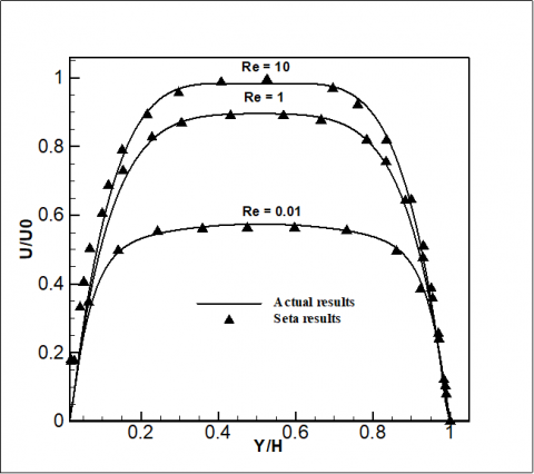
The inlet and the outlet positions are respectively $\mathrm{x}_{1}$ and $\mathrm{x}_{\mathrm{n}}$ The Reynolds number of Poiseuille flow $\mathrm{Re}$ is given by $\operatorname{Re}=\frac{\mathrm{Hu}_{0}}{v}$ where $\mathrm{u}_{0}$ refers to the peak velocity of the flow along the centerline of the channel [5-7]. The Darcy number is defined by $=\frac{\mathrm{K}}{\mathrm{H}^{2}}$ . The porosity is fixed to 0.1 and the Rayleigh number is equal to 0.1. Initially the velocity field is zero at each node. The resolution of equation (12) is made by applying the second order finite difference scheme with a uniform mesh (FDM). The grid size dependence is studied at different Reynolds number. The maximum velocity and pressure are compared. The results are shown in the Table1. The maximum change of using finer mesh is about 1.2%. The results are grid independent.  In the Figures 1 and 2 the velocity profiles for different values of Reynolds and Darcy are compared with Seta numerical results. These results are also verified by the FDM solutions. The Figure shows an agreement between the present results and the Seta work [6].

For more accuracy the root mean square error (RMSE) is calculated by the following equation:

$\sqrt{\frac{\sum_{1}^{\mathrm{z}}\left(\mathrm{M}_{\mathrm{LBM}}-\mathrm{M}_{\theta}\right)^{2}}{\mathrm{Z}}}$(14)

Figure 1 and figure 2 present a good agreement with Seta results for different Reynolds number and Darcy number of the velocity for poiseuille flow.

figure_1.png

Figure 1. Velocity profile of the Poiseuille flow for different Reynolds number

Table 1. Grid dependence at different Reynolds number

figure_2.png

Figure 2. Velocity profile of the Poiseuille flow for different Darcy number

The Table 2 gives the RMSE between the LBM results and the Seta work at different Reynolds.

Table 2. The RMSE at different Reynolds number

The Table 3 gives the RMSE between the LBM results and the Seta work at different Darcy number.

Table 3. The root mean square error at different Darcy number

4.2 Thermal injected flows

The second case is a hot fluid sheared in a porous channel. It was injected normal to the shearing direction. The upper and lower plates are fixed and kept at a constant temperature respectively $\mathrm{T}_{\mathrm{h}}$ and $\mathrm{T}_{\mathrm{c}}$. On the inlet and the upper side the Zou and He work are applied to calculate the dynamic boundary. In the inlet, the unknown functions and the density are:

$\rho_{i n}=\frac{1}{1-u_{i n}}\left[f_{0}+f_{2}+f_{4}+2\left(f_{3}+f_{6}+f_{7}\right)\right]$(15)

$\left\{\begin{array}{c}{f_{1}=f_{3}+\frac{2}{3} \rho_{i n} u_{i n}} \\ {f_{7}=f_{5}-\frac{1}{2}\left(f_{2}-f_{4}\right)+\frac{1}{6} \rho_{i n} u_{i n}+\frac{1}{2} \rho_{i n} v_{i n}} \\ {f_{8}=f_{6}+\frac{1}{2}\left(f_{2}-f_{4}\right)+\frac{1}{6} \rho_{i n} u_{i n}+\frac{1}{2} \rho_{i n} v_{i n}}\end{array}\right.$(16)

On the bottom we use the bounce back conditions. For The thermal boundary conditions we resort to the Direchlet condition given by the following equation:

$g_{i}=T_{k}\left(\omega_{i}+\omega_{i+2}\right)-g_{i+2}$(17)

If the Forchheimer term is neglected the flow is governed at steady state by:

$\frac{v_{e}}{\varepsilon} \frac{\partial^{2} u}{\partial y^{2}}+G_{x}-\frac{v}{K} u=0$(18)

Where $G_{x}=-g_{0} \beta\left(T-T_{m}\right)+a_{y}$

The term $a_{y}$ is:

$a_{y}=\frac{v}{K} v_{0}-g_{0} \beta \Delta T\left[\frac{\exp \left(\frac{y v_{0}}{\alpha}\right)-1}{\exp \left(\frac{H v_{0}}{\alpha}\right)-1}\right]$(19)

The temperature satisfies the energy equation (equation (8)). At steady state the analytics solutions for velocity and temperature are expressed as follows:

$u=u_{0} \exp \left[r\left(\frac{y}{H}-1\right)\right] \frac{s h\left(\frac{C y}{H}\right)}{s h(c)}$(20)

$T=T_{h}+\Delta T \frac{\exp \left(\frac{P r * R e * y}{H}\right)-1}{\exp (\operatorname{Pr} * \operatorname{Re})-1}$(21)

$r, C$ and $\Delta T$ are respectively given by $r=\frac{R e}{2 \varepsilon} C=\frac{1}{2 \varepsilon} \sqrt{R e^{2}+\frac{4 \varepsilon}{D a}}$ and $\Delta T=T_{h}-T_{c}$.

The Rayleigh and Prandlt numbers are respectively 100 and 1. The porosity is equal to 0.7. The Darcy number is chosen to be 0.1 and the Reynolds number changes from 1 to 50. The grid independence of the results is established for different Reynolds numbers. The magnitude of the maximum $x$ and $y$-velocity along the horizontal centerline and the maximum of pressure with changing grid size are shown in the Table 4.

Table 4. Grid dependence at different Reynolds number

figure_3a.png

(a) Velocity profile

figure_3b.png

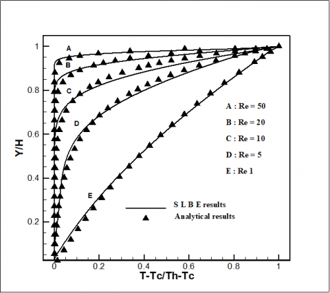
(b) Temperature profile

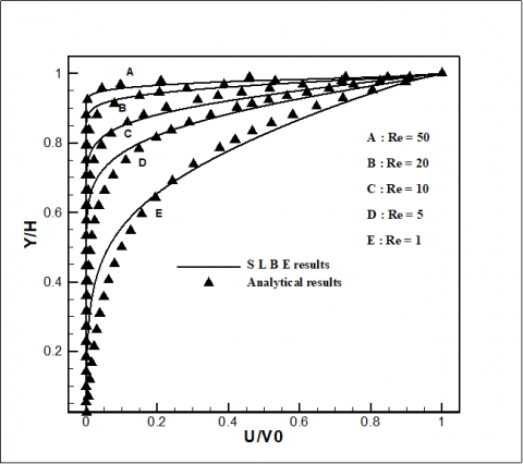
Figure 3. Velocity and temperature profiles for different Reynolds number, SLBE and analytical simulations

The Figure 3(a) proves that when Re increases the porous media resistance to velocity fields becomes more important. The velocity layer thickness decreases by approaching to the moving wall. The Figure 3(b) shows that the increment of Reynolds number generates the decline of temperature. This is due to the strength convection in the channel when Re is large. More heat will be taken away by the flow.

The figure 3(b) presents a good agreement with asymptotic solution. For different Reynolds number the velocity and the temperature RMSE between the LBM results and the analytical values are established. The results are given in Table 5.

Table 5. Velocity and temperature root mean square error

figure_4.png

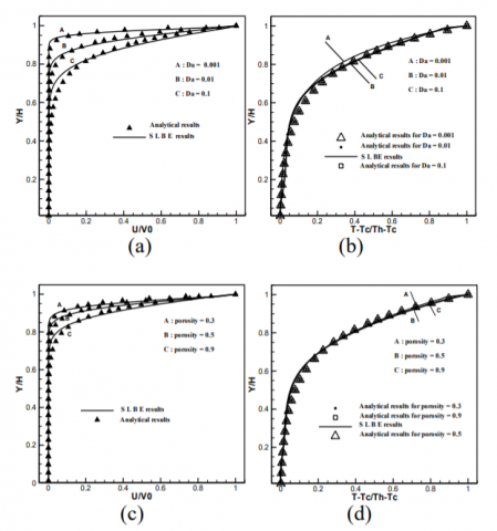
Figure 4. Velocity and temperature profiles for different Darcy number and porosity, the solid lines are SLBE results and the symbols are analytical solutions; (a, c) velocity profile (b, d) temperature profile

The Figure 4(a) shows that the increment of $\mathrm{Da}$ is accompanied by the rise of the flow velocity. The flow attitude tends towards that of a free media. The velocity profile becomes more linear. The Figure 4(b) shows that there is an infinitesimal difference between the temperature profiles. This is interpreted by the negligible effect of horizontal flow. The heat transfer is vertical from bottom to top. For Reynolds and Darcy equal to 5 and 10^-2, the porosity changes from 0.3 to 0.99. The Figure 4(c) shows that the porosity increment allows fluid flow readily. The porous medium drags decreases. The Figure 4(d) proves that the porosity change didn’t engender notified difference on the temperature profile.

The Table 6 describes the velocity and the temperature root mean square error between LBM results and the analytic values

Table 6. Root mean square at different porosity

4.3 GLBE and SLBE comparison

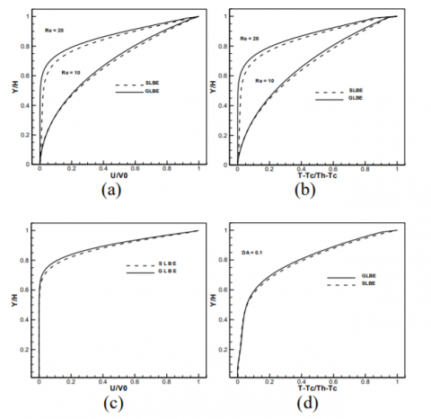
The inertia drags is modulated by Forchheimer term. Its effect on fluid flow and heat transfer is studied. So the previous study is performed using the GLBE We follow for each parameter the evolution of velocity and temperature values at a lattice node and the cross section (X=0.5). The GLBE and SLBE results are compared. The Figure 5 shows the velocity and temperature results at different dynamic parameter for a lattice node.

figure_5.png

Figure 5. GLBE and SLBE results for different porosity, Reynolds and Darcy

The Figures 6 shows the velocity and temperature profiles at the lattice cross section $X=0.5$. The results are given at different Reynolds and Darcy number. Through the above Figures, the $D a$ or $R e$ increment hinders the flow and the heat transfer. This is caused by the nonlinear drag force. This is observed also if the porosity decreases. Therefore, for small Darcy and Reynolds number the simulation can be restricted to the SLBE approach. For large value the Forchheimer term should not be neglected. The RMSE between the GLBE and SLBE determine the critical Reynolds and Darcy number for the selection of GLBE. Indeed, when $R M S E \leq 10^{-3}$ the SLBE is sufficient. In this case, the comparison shows that the critical values of respectively the Reynolds and Darcy number are less than 1 and 10^-2.

figure_6.png

Figure 6. Velocity and temperature profile using GLBE and SLBE for different Reynolds and for Darcy=0.1, (a, c) velocity profile (b, d) temperature profile

4.4 Thermal flow in porous plate with fixed wall

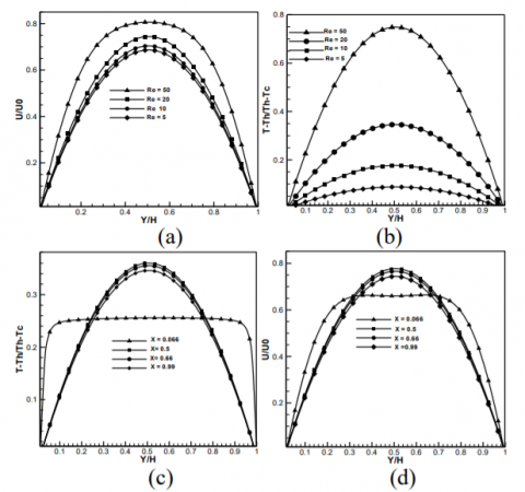
The geometry of the problem consists in a hot fluid forced to flow into a planar channel filled with porous media. The upper and lower plates are fixed and kept at a constant temperature $T_{c}$. On the left the distribution functions are established thanks to Zou and He conditions [19]. In the upper and lower solid wall, the distribution functions are given by the no slip boundary conditions. For the thermal boundary, we resort to Dirichlet expressions (Eq(17)). The GLBE model is chosen for simulation. The velocity and the temperature profiles are plotted for different Reynolds number (Figure 7). The dynamic and thermal flow behavior inside the channel is described. The velocity and the temperature are plotted at different sections.

figure_7.png

Figure 7. Velocity and temperature profiles for different Reynolds in different cross section, (a, d) velocity profile (b, c) temperature profile

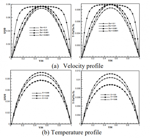
The variation of Darcy number affects the velocity and the temperature. The results are presented in the Figure 8. When $D a$ is equal to 10^-3 the flow is followed inside the porous channel. The temperature and the velocity at different cross sections are presented.

figure_8.png

Figure 8. Velocity and temperature profiles for different Darcy number and at different cross sections, (a, c) velocity profile (b, d) temperature profile

Table 7. The evolution of the average Nusselt number and permeability at different porosity

In these models, the solid fraction determines the local permeability at each node. Here, we measure the permeability of the different models by applying a pressure differential across a domain filled with nodes of a single solid fraction. The isotropic (thus scalar) intrinsic permeability $K$ is calculated from Darcy’s law.

$K=\frac{\varepsilon^{3} d_{p}^{2}}{150(1-\varepsilon)^{2}}$(22)

$d_{p}$: The solid particle diameter.

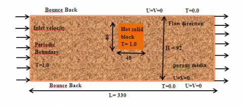
4.5 Heat transfer and fluid flow in porous media containing hot obstacle

The problem consists of a hot fluid flow in porous channel containing hot obstacle Figure 9.

figure_9.png

Figure 9. Scheme of flow in the porous channel

The presence of the hot block requires the use of the Dirichlet boundaries for thermal conditions. For the dynamic conditions the Bounce back boundaries are applied. For all the simulation the previous circumstances are kept. The results at different factors are given by the following Figures.

The Figure 10 reports the sensibility to the porosity variation. For lower porosity the temperature of the fluid increases. This can be explained by the increment of the thermal conductivity by the porosity decrease. The increment of the porosity leads to a slight rise of velocity at the top and bottom of the block. The increment of the porosity makes easier for the fluid to vary its paths to the upper and bottom wall. Thus the velocity increases on the walls.

figure_10.png

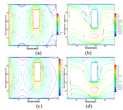
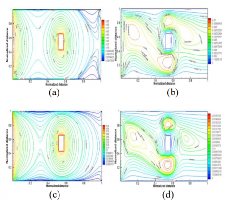
Figure 10. Temperature and velocity contours for different porosity respectively 0.5 and 0.9 at 6000 time step; (a, c) temperature (b, d) velocity contours

figure_11.png

Figure 11. Temperature and velocity contours for different Darcy number respectively 10^-4 and 10^-5 at 8000 time step; (a, c) temperature (b, d) velocity contours

Secondly the sensibility of the Darcy number is studied (Figure 11). Through this Figure, the Darcy variation affects the heat transfer and especially the velocity field. Their independence is due to constant properties of the flow. The increment of the Darcy generates an infinitesimal increase of the fluid temperature and the heat transfer. The velocity field increases due to the large permeability values.The velocity and temperature contours for different Reynolds number are plotted in Figure 12. As the Reynolds number increases the velocity of the flow increases. Consequently, the convective coefficient and the magnitude of heat transfer increase. For high Reynolds number the medium temperature wanes due to the decrease in the heat transfer process.

figure_12a.png

figure_12b.png

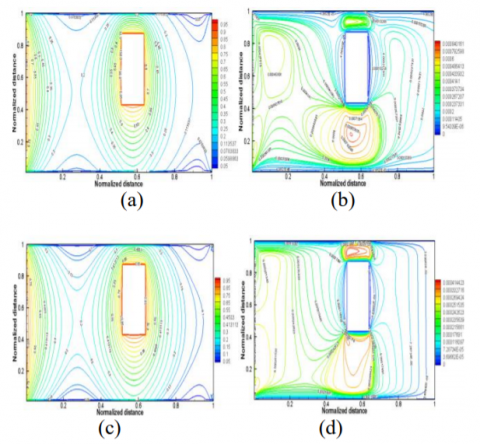
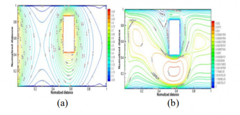
Figure 12. Temperature and velocity contours for different Reynolds number respectively 5 and 20 at 8000 time step; (a, c) temperature (b, d) velocity contours

figure_13.png

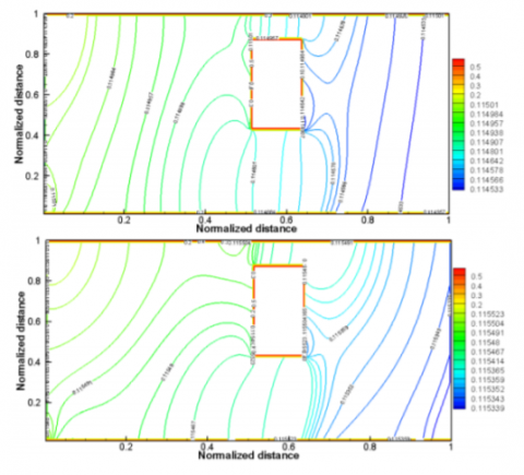
Figure 13. Pressure contours at different Reynolds number respectively 20 and 5

The Figure 13 shows the pressure distribution in the porous medium at different Reynolds number. The high pressure region is significantly increased in upstream zone, which extends over obstacle. The velocity vector fields at different Reynolds number is given by the Figure 14. These results indicate that the obstacle strength plays an important role to increase the intensity of velocity magnitude in the obstacle bottom and top zone.

figure_14.png

Figure 14. Velocity vectors field and vortices for different Reynolds number respectively 20 and 5

figure_15.png

Figure 15. Temperature and velocity contours at different Reynolds number respectively 5 and 20 at 8000 time step; (a, c) temperature (b, d) velocity contours

It is clear from the velocity vector plots in Figure 14 that the zone near obstacle will be a region of strong axial vortices, at least in cross flow, adjacent the obstacle there are small regions of concentrated vortices. The effect of the obstacle dimension and the position is studied for different Reynolds number. The length and width are 20 cm. It is placed in the channel center. Figure 15 shows the isotherms and the velocity contours. The obstacle suitable distances from the wall. Hence, the boundaries conditions do not affect the flow. The influence of the obstacle is well appeared. As a result, the dimensionless temperature and velocity contours are significantly different for these two cases with different obstacle dimensions