OPEN ACCESS
Stability and transition problems of two dimensional laminar external flow over a flat plate with wall suction and blowing are studied numerically using the temporal linear stability theory. The flow is assumed similar two-dimensional laminar boundary-layer. The mean velocity profiles are obtained numerically for the case of suction or blowing. The stability equation is given in a general form which can be applied to Chebyshev domain and in boundary layer domain and solved numerically by the Chebyshev collocation spectral method. The neutral stability curves and the critical Reynolds numbers are presented.
External flow, Stability, Suction, Blowing, Collocation spectral method.
Instability of laminar external flow and their transition to turbulence are important phenomena in many engineering flow systems. Researchers have studied these occurrences for decades, focusing on how external agents, such as free-stream fluctuations and wall roughness, induce boundary-layer disturbances, and on whether the latter become unstable and lead to the laminar flow breakdown [1]. About 50% of the drag of a modem commercial aircraft is caused by skin friction. Due to the fact that turbulent boundary layers produce higher drag than laminar layers, the delay of transition is of particular interest. Several strategies to stabilize laminar flow have been investigated extensively, such as suction, mean flow distortion and wave cancellation by superposition [2, 3].
A direct numerical simulation of the effects of uniform blowing or suction from a spanwise slot on a turbulent boundary layer has been investigated by Park and Choi [4]. The authors showed that application of small-magnitude uniform blowing and suction significantly changes the skin friction and turbulence intensities above the slot as well as downstream of the slot. For both cases of blowing and suction, the streamwise turbulence intensity recovers quickly from blowing or suction, while other components of the turbulence intensities and Reynolds shear stress recover in a longer downstream distance .
Ricco and Dilib [5] deals with the effects of distributed steady wall suction and blowing on a Blasius boundary layer perturbed by low-frequency, streamwise-elongated vertical disturbances induced by free-stream vertical perturbations.
Kim et al. [6] examined the effect of blowing velocity on the characteristics of the turbulent boundary layer. They conducted direct numerical simulations at three values of the blowing velocity under conditions of constant mass flow rate through the slot.
Mehrez et al. [7] analysed numerically by Large Eddy Simulation (LES) methodology the effects of local perturbation on the dynamic structure and heat transfer in turbulent separated and reattached flow over a backward-facing step. The perturbation is imposed by a local sinusoidal blowing/suction of the fluid into a separated shear layer. The simulation results show the existence of an optimum perturbation frequency value where the maximum enhancement of heat transfer is observed.
Ahmed and Kalita [8] investigated the free convective oscillatory flow of a viscous incompressible and electrically conducting fluid past a vertical porous plate in sleep flow regime with variable suction and periodic plate temperature in presence of a uniform transverse magnetic field. Analytical solutions to the coupled non-linear equations governing the flow and heat transfer are derived by using perturbation method with Eckert number as perturbation parameter. The amplitudes and the phases of the fluctuating parts of the skin friction and heat transfer at the plate are shown graphically.
Kim and Sung [9] performed direct numerical simulations of a spatially evolving turbulent boundary layer to study the effect of periodic blowing at a fixed frequency on a turbulent boundary layer. By comparing the flow behavior of the system under steady flow conditions with that in the presence of periodic blowing, they showed that periodic blowing causes the enhancement of energy redistribution of turbulence intensities near the wall.
Generally, the linear stability of hydrodynamic problems is governed by the Orr-Sommerfeld equation. For parallel shear flows with homogeneous boundary conditions, this equation constitutes an eigenvalue problem. For temporally evolving flows, the eigenvalue is the complex frequency and the problem becomes linear in the eigenvalue. Although for small amplitude disturbances, temporal evolution is a good approximation to the laboratory flow, the correct physics of the problem can be obtained only through the calculation of spatially evolving modes. In the Orr-Sommerfeld equation, these modes are given in terms of the wave number and for these situations, where the complex wave number is the eigenvalue, the Orr-Sommerfeld equation becomes a nonlinear eigenvalue problem.
Since the pioneering work of Orszag [10] in 1971, spectral methods have emerged as a powerful tool to solve hydrodynamic stability problems. Orszag applied a Chebyshev tau technique to transform the Orr-Sommerfeld equation for plane Poiseuille flow to a matrix generalized eigenproblem $K u=\gamma M u$, solved at Reynolds numbers of order 104 using the QR algorithm. The superior performance of the Chebyshev tau method compared to existing finite-difference and spectral schemes led to its application to a diverse range of stability problems [11].
Dongarra et al. [12] and Melenk et al. [13] consider a general mathematical framework spectral methods for hydrodynamic stability problems. They analyze the Orr–Sommerfeld equation supplied with homogeneous boundary.
The pseudospectra and the numerical range of this Orr–Sommerfeld operator is also investigated by Reddy, Schmid and Henningson [14].
Hifdi et al. [15] present a temporal linear stability analysis of symmetric developing flows slightly perturbed from Poiseuille flow. The Chebyshev spectral collocation method is used to solve the Orr–Sommerfeld equation. For the mean flow, the solution considered is analytic. The results of the stability study depend essentially on the shape and amplitude of the velocity profiles imposed at the channel entry.
In the present study, the hydrodynamic linear stability of external flow over a flat plate with wall suction or blowing is investigated. The flow is assumed similar two-dimensional laminar boundary-layer. The mean velocity profiles are obtained numerically for the case of suction or blowing. The eigenvalue problem associated with the Orr-Sommerfeld stability equation is solved to high accuracy by employing Chebyshev collocation spectral method. The numerical solutions facilitate the construction of complete neutral stability curves and the determination of stability characteristics for a wide range of permeable wall intensities extending from strong blowing to strong suction.
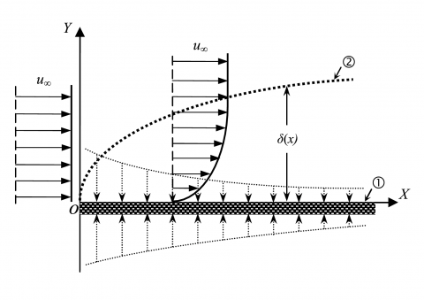
A schematic diagram of the physical problem is shown in Figure 1. It consists of permeable wall, in direct contact with laminar external flow. The physical model is two-dimensional. The coordinates system OXY is located on the plate and defined as: OX axis is in the flow direction, OY axis is normal to the plate and directed towards the flow.
Figure 1. Schematic diagram of the physical problem ① wall with suction (↑) or blowing (↓); ② laminar boundary layer
Laminar two-dimensional external flow is governed by the Navier-Stokes equations
$\frac{\partial u}{\partial X}+\frac{\partial v}{\partial Y}=0$(1)
$\frac{\partial u}{\partial t}+u \frac{\partial u}{\partial X}+v \frac{\partial u}{\partial Y}=-\frac{1}{\rho} \frac{\partial p}{\partial X}+v\left(\frac{\partial^{2} u}{\partial X^{2}}+\frac{\partial^{2} u}{\partial Y^{2}}\right)$(2)
$\frac{\partial v}{\partial t}+u \frac{\partial v}{\partial X}+v \frac{\partial v}{\partial Y}=-\frac{1}{\rho} \frac{\partial p}{\partial Y}+v\left(\frac{\partial^{2} v}{\partial X^{2}}+\frac{\partial^{2} v}{\partial Y^{2}}\right)$(3)
The boundary conditions are defined as
At the wall (Y=0)
$u=u_{w}$(4)
$v=v_{w}(X)$(5)
At outside border of boundary layer ($Y \rightarrow \infty$)
$u=u_{\infty}$(6)
The stability of parallel shear flows under two-dimensional infinitesimal disturbances of the form $\tilde{\psi}(x, y, \tau)=\varphi(y) e^{i \alpha(x-c \tau)}$ is governed by the Orr-Sommerfeld equation (the derivation of this equation is given in the Appendix).
$\varphi^{\prime \prime \prime \prime}-2 \alpha^{2} \varphi^{\prime \prime}+\alpha^{4} \varphi-i \alpha \operatorname{Re}\left[(U-c)\left(\varphi^{\prime \prime}-\alpha^{2} \varphi\right)-U^{\prime \prime} \varphi\right]=0$(7)
with the conditions
$\varphi=\varphi^{\prime}=0 \quad$ at $\quad y=0, y \rightarrow \infty$(8)
where superscripts indicate derivatives with respect to y, Re is the Reynolds number, $\varphi(y)$ is the complex amplitude of the wave $\psi(x, y, \tau)$, U is the mean flow dimensionless velocity profile and a and c the wave number and the complex wave velocity, respectively.
The quantities $\varphi$ and c are defined as
$\varphi=\varphi_{r}+i \varphi_{i}$(9)
$c=c_{r}+i c_{i}$(10)
The real part of c represents the wave phase velocity while the imaginary part ci determines the attenuation or amplification of disturbances. The flow is stable, neutrally stable, or unstable depending on whether ci is negative, zero, or positive.
The solution of stability equation (7) depends on the mean velocity profile U. For laminar boundary layer over a flat plate with suction or blowing, this quantity is not known explicitly, but it is obtained numerically from the nonlinear ordinary differential Blasius equation
$\frac{d^{3} f}{d \xi^{3}}+\frac{1}{2} f \frac{d^{2} f}{d \xi^{2}}=0$(11)
subject to the boundary conditions
$\frac{d f}{d \xi}(0)=0$(12)
$f(0)=f_{w}$(13)
$\frac{d f}{d \xi}(\infty)=1$(14)
where $\xi$ is the similarity coordinate and f the non dimensional stream function given by Skan-Falkner transformation:
$\xi=Y \sqrt{\frac{u_{\infty}}{\nu X}}$(15)
$f=\frac{\Psi}{u_{\infty} \sqrt{(\nu X) / u_{\infty}}}$(16)
In terms of similarity coordinate and stream function, dimensionaless axial and normal velocity components are:
$U=\frac{d f}{d \xi}$(17)
$V=\frac{1}{2 u_{\infty}} \sqrt{\frac{\nu u_{\infty}}{X}}\left(\xi \frac{d f}{d \xi}-f\right)$(18)
At the wall, the normal velocity component is:
$V_{w}=-\frac{1}{2 u_{\infty}} \sqrt{\frac{\nu u_{\infty}}{X}} f_{w}$(19)
From this equation, we note that flow blowing, produced by imposing inward parietal velocity, is characterized by negative values of wall stream function. While flow suction, produced by imposing outward parietal velocity, is characterized by positive values of stream function.
The mean velocity profile for a similar laminar boundary-layer over a flat plate with wall suction and blowing characterized by constant wall stream function is obtained numerically by solving equation (11) using Runge-Kutta method (RK-4).
The Chebyshev spectral collocation method is applied to solve the stability Equation (7). A complete and broad description of Chebyshev spectral methods is given in [16-19]. This method is based on the Chebyshev polynomials of order k defined on the interval [-1, 1] by
$T_{k}(\eta)=\cos \left(k \cos ^{-1} \eta\right) ; \quad k=0,1, \ldots, N$(20)
The Gauss-Lobatto collocation points [17-18] is used to define the Chebyshev nodes in the domain [-1, 1], namely
$\eta_{j}=\cos (\pi j / N),-1 \leq \eta \leq 1, \quad j=0,1,2, \ldots N$(21)
where N is the number of intervals and $\eta$ represents the coordinates of the collocation points in the Chebyshev domain.
The physical quantity $\varphi(y)$ is approximated by the interpolating polynomial in terms of the collocation points by employing the truncated Chebyshev series of the form
$\varphi(\eta)=\sum_{k=0}^{N} a_{k} T_{k}(\eta)$(22)
This expression can be expressed as
$\varphi(\eta)=\sum_{k=0}^{N} C_{k}(\eta) \varphi\left(\eta_{k}\right)$(23)
where the expansion coefficients Ck may be evaluated by
$C_{k}(\eta)=\frac{2}{N b_{k}} \sum_{m=0}^{N} \frac{1}{b_{m}} T_{m}\left(\eta_{k}\right) T_{m}(\eta)$(24)
where
$\left\{\begin{aligned} b_{k}=1 &(k=1,2, \ldots \ldots, N-1) \\ b_{0} &=b_{N}=2 \end{aligned}\right.$(25)
The nth derivative of $\varphi_{N}(\eta)$ is then approximated by the following expression.
$\varphi^{(n)}(\eta)=\sum_{k=0}^{N} C_{k}^{(n)}(\eta) \varphi\left(\eta_{k}\right)$(26)
where n is the order of differentiation.
Derivatives of the variables at the collocation points may be represented by
$\varphi^{(n)}\left(\eta_{j}\right)=\sum_{k=0}^{N} C_{k}^{(n)}\left(\eta_{j}\right) \varphi\left(\eta_{k}\right)$(27)
The first derivative at the Chebyshev-Gauss-Lobatto points satisfy
$C_{k}^{(1)}\left(\eta_{j}\right)=d_{j k}$(28)
where djk are the elements of the Chebyshev spectral differentiation matrix D defined as [16-17].
$\left\{\begin{array}{c}{d_{00}=-\frac{2 N^{2}+1}{6}} \\ {d_{N N}=-d_{00}} \\ {d_{k j}=\frac{b_{k}}{b_{j}} \frac{(-1)^{k+j}}{\eta_{k}-\eta_{j}} \quad(k \neq j)} \\ {d_{j j}=-\frac{\eta_{j}}{2\left(1-\eta_{j}^{2}\right)}}\end{array}\right.$(29)
Now, the discrete values of the first derivative of the function $\varphi^{\prime}\left(\eta_{j}\right)$ can be obtained as follows
$\varphi^{(1)}\left(\eta_{j}\right)=\sum_{k=0}^{N} d_{j k} \varphi\left(\eta_{k}\right)$(30)
This equation can be written in matrix-vector form as follows
$\tilde{\varphi}^{(1)}=\mathrm{D} \hat{\varphi}$(31)
where
$\left\{\begin{aligned} \hat{\varphi}^{(1)} &=\left(\varphi^{(1)}\left(\eta_{0}\right), \ldots, \varphi^{(1)}\left(\eta_{N}\right)\right)^{T} \\ \widehat{\varphi} &=\left(\varphi\left(\eta_{0}\right), \ldots, \varphi\left(\eta_{N}\right)\right)^{T} \end{aligned}\right.$(32)
The second-order derivative expansion is
$\varphi^{(2)}\left(\eta_{j}\right)=\sum_{k=0}^{N} C_{k}^{(2)}\left(\eta_{j}\right) \varphi\left(\eta_{k}\right)$(33)
This is written in matrix form as
$\widehat{\varphi}^{(2)}=\mathrm{D}^{(2)} \widehat{\varphi}$(34)
where
$\widehat{\varphi}^{(2)}=\left(\varphi^{(2)}\left(\eta_{0}\right), \ldots, \varphi^{(2)}\left(\eta_{N}\right)\right)^{T}$(35)
The second derivative matrix $D^{(2)}$ can be obtained analytically using an explicit expression or by the following relation $D^{(2)}=D \times D([19])$.
In the present study, relating boundary layer flow problem, the calculations require the mapping of the physical domain onto the Chebyshev domain. The wall-normal domain varies in the range [0,y∞], where y∞ is the outside border of boundary layer. To transform Chebyshev interval -1 ≤ η ≤ 1 into the computational domain 0 ≤ y ≤ y∞ , Motsa and Makukula [22] derived a grid transformation that mapped the Chebyshev collocation points to a new set of interpolation points. The grid transformation was defined as
$y=y_{\infty} \frac{1+\eta}{2}$(36)
Therefore,
$\left\{\begin{array}{ll}{y=0} & {\text { for } \quad \eta=-1} \\ {y=y_{\infty}} & {\text { for } \quad \eta=1}\end{array}\right.$(37)
and the derivative of $\varphi(y)$ is then evaluated as
$\left\{\begin{array}{l}{\frac{d \varphi}{d y}=\frac{d \varphi}{d \eta} \frac{d \eta}{d y}=\frac{2}{y_{\infty}} \frac{d \varphi}{d \eta}} \\ {\varphi^{(1)}\left(y_{j}\right)=\frac{2}{y_{\infty}} \varphi^{(1)}\left(\eta_{j}\right)} \\ {\varphi^{(n)}\left(y_{j}\right)=\frac{2}{y_{\infty}} \varphi^{(n)}\left(\eta_{j}\right)}\end{array}\right.$(38)
With a definition of a new differentiation matrix $\widehat{D}$ with D being the Chebyshev spectral differentiation matrix.
$\widehat{D}=\left(2 / y_{\infty}\right) D$(39)
The first and second derivative matrix expressed at the collocation points of the physical domain can be represented in matrix-vector form as follows.
$\left\{ \begin{matrix} {{{\overset{\scriptscriptstyle\frown}{\varphi }}}^{(1)}}={\overset{\scriptscriptstyle\frown}{D}}\overset{\scriptscriptstyle\frown}{\varphi } \\ {{{\overset{\scriptscriptstyle\frown}{\varphi }}}^{(2)}}={{{{\overset{\scriptscriptstyle\frown}{D}}}}^{(2)}}\overset{\scriptscriptstyle\frown}{\varphi } \\ {{{\overset{\scriptscriptstyle\frown}{\varphi }}}^{(1)}}={{({{\varphi }^{(1)}}({{y}_{0}}),....,{{\varphi }^{(1)}}({{y}_{N}}))}^{T}} \\ {{{\overset{\scriptscriptstyle\frown}{\varphi }}}^{(2)}}={{({{\varphi }^{(2)}}({{y}_{0}}),....,{{\varphi }^{(2)}}({{y}_{N}}))}^{T}} \\ \end{matrix} \right.$ (40)
It is now convenient to write the Orr-Sommerfeld equation (7) in a different form
$\left[\left(\widehat{D}^{(2)}-\alpha^{2} I\right)^{2}-i \alpha \operatorname{Re}\left\{(U I-c I)\left(\widehat{D}^{(2)}-\alpha^{2} I\right)-U^{\prime \prime} I\right\}\right] \varphi=0$(41)
where I is the identity matrix of order N×N.
We note that this equation can be applied in both domains. By taking:
Equation (41) is a polynomial in α with matrix coefficients and has the following explicit form,
$P_{4}(\alpha) \varphi=\left(C_{0} \alpha^{4}+C_{1} \alpha^{3}+C_{2} \alpha^{2}+C_{3} \alpha+C_{4}\right) \varphi=0$(42)
where the matrix coefficients are
$\left\{ \begin{matrix} {{C}_{0}}=I \\ {{C}_{1}}=i\operatorname{Re}\left( UI-cI \right) \\ {{C}_{2}}=-2{{{\overset{\scriptscriptstyle\frown}{D}}}^{(2)}}I \\ {{C}_{3}}=-i\operatorname{Re}U{{{\overset{\scriptscriptstyle\frown}{D}}}^{(2)}}+i\operatorname{Re}c{{{\overset{\scriptscriptstyle\frown}{D}}}^{(2)}}+i\operatorname{Re}{{U}'}'I \\ {{C}_{4}}={{{\overset{\scriptscriptstyle\frown}{D}}}^{(4)}} \\ \end{matrix} \right.$(43)
Different numerical methods can be used to solve equation (42). The simplest one consists in transforming it to a linear problem of larger dimension by forming the so-called companion matrices [20]. A companion matrix for equation (42) can be written as
$\left[\left(\begin{array}{cccc}{-C_{1}} & {-C_{2}} & {-C_{3}} & {-C_{4}} \\ {I} & {0} & {0} & {0} \\ {0} & {I} & {0} & {0} \\ {0} & {0} & {I} & {0}\end{array}\right)-\alpha\left(\begin{array}{cccc}{C_{0}} & {0} & {0} & {0} \\ {0} & {I} & {0} & {0} \\ {0} & {0} & {I} & {0} \\ {0} & {0} & {0} & {I}\end{array}\right)\right]\left[\begin{array}{c}{\alpha^{3} \varphi} \\ {\alpha^{2} \varphi} \\ {\alpha^{1} \varphi} \\ {\varphi}\end{array}\right)=0$(44)
This equation constitutes a generalized eigenvalue problem for α, and can be solved efficiently by the QZ-algorithm [10].
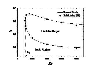
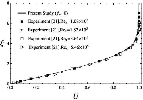
In Figures 2 and 3, the neutral stability curve and the mean flow velocity profile obtained in this study are compared with experimental results reported in the literature for impermeable wall (fw=0), [21]. A good agreement is observed. The neutral stability curve corresponds to ci=0. It separates the unstable region (ci>0) and the stable region (ci<0), that remain inside and outside this curve.
Figure 2. Neutral stability curve for impermeable wall: - numerical results, ■ experience [21]
Figure 3. Velocity profile for impermeable wall: - numerical results, ■ experience [21]
Table 1 shows a comparison between obtained eigenvalues using various methods for the case Re=580, α=0.179, y∞=20 and N+1=44. The eigenvalues are given for the single unstable mode (ci>0). This comparison shows that the present numerical method is accurate.
Table 1. Eigenvalues of the Orr-Sommerfeld equation for laminar boundary layer (fw=0), Re=580, α=0.179
|
Results |
Eigenvalues |
|
Present study Grosch and Orszag [23] Zebib [24] Hatziavramidis and Ku [25] Xie et al. [26] |
0.364552+0.0077791i 0.364557+0.007773i 0.364143+0.007959i 0.364372+0.007884i 0.36455 +0.0077793i |
7.1 Mean velocity profiles
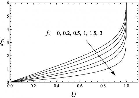
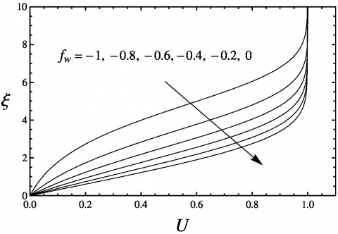
Figures 4 and 5 present the mean velocity profiles obtained numerically by solving Equation (11) with the boundary conditions given in Equations (12)-(14) by standard Runge-Kutta method. Mathematically, suction or blowing are produced by imposing positive or negative values of wall stream function, respectively. We note that, the dimensionless velocity decreases with increasing the intensity of suction and increases with increasing the intensity of blowing. The intensity of suction or blowing is defined as the absolute value of the wall stream function.
Figure 4. Mean velocity profile for wall suction (fw>0)
Figure 5. Mean velocity profile for wall blowing (fw<0)
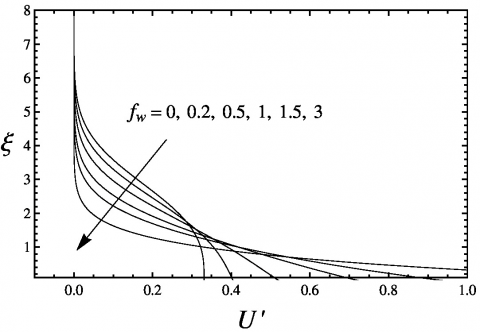
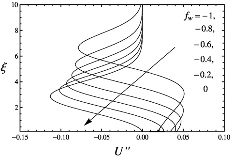
Figure 6. Velocity first-order derivative for wall suction
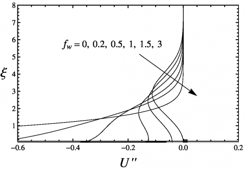
Figure 7. Velocity second-order derivative for wall suction
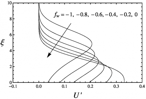
Figure 8. Velocity first order derivative for wall blowing
Figure 9. Velocity second-order derivative for wall blowing
The distributions of the first-order derivative U’ and the second-order derivative U'' of the velocity for the case of suction or blowing are shown in Figure 6 to 9, respectively. These quantities play an important role in the stability phenomena, and to achieve accurate results of the stability calculations, these profiles have to be produced with great accuracy.
7.2 Stability and transition characteristics of flow
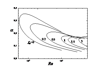
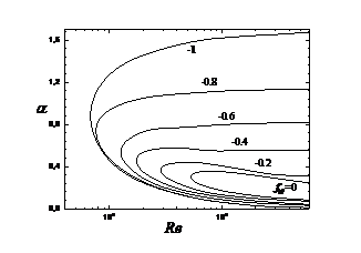
Neutral stability curves are presented in the (Re, α) plan for some values of the wall stream function, as can be seen in Figures 10 and 11.
In the neutral stability curves for suction, Figure 10, one sees a marked shifting to the right as the intensity of the suction increases. That is, the region of flow stability extends to higher Reynolds numbers as the suction becomes stronger.
In Figure 11, it is seen that increase in the intensity of blowing cause a marked left ward change of the curves, that is, toward lower Reynolds numbers. Thus, blowing is seen to be highly destabilizing.
Figure 10. Neutral stability curves, for wall suction (fw>0)
Figure 11. Neutral stability curves, for wall blowing (fw<0)
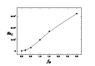
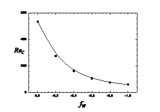
The summary of the stability calculations for two dimensional laminar external flow over a flat plate with wall suction and blowing submitted to linear two-dimensional disturbances is presented in Figure 12 and 13. Here the variation of the critical Reynolds number with suction and blowing is illustrated. As it is evident from this figures, the critical Reynolds number increases with increasing the intensity of suction or decreasing the intensity of blowing.
Figure 12. Critical Reynolds numbers for suction
Figure 13. Critical Reynolds numbers for blowing
This study is focused on the temporal linear stability characteristics of laminar forced convection external flows along a horizontal permeable flat plate. For the mean flow, the similar boundary layer equations are used and solved numerically by a point-by-point Runge-Kutta-Verner method. The eigenvalue problem for the disturbance flow was solved numerically by the Chebyshev collocation spectral method. Neutral stability curves and critical Reynolds numbers are presented for different values of the wall stream function fw ranging from 0.2 to 3 for wall suction and from -0.2 to -1 for wall blowing. The numerical solutions indicate the important role of the suction or blowing effect on the stability characteristics. The critical Reynolds number increases with increasing the intensity of suction or decreasing the intensity of blowing.
|
c |
complex wave velocity |
|
Ci |
matrix coefficients, defined in Eq. (43) |
|
D |
the Chebyshev spectral differentiation matrix. |
|
djk |
elements of the Chebyshev spectral differentiation matrix Eq. (29) |
|
f |
non-dimensional stream function |
|
i |
complex number |
|
I |
identity matrix |
|
L |
length scale [m] |
|
N |
number of intervals in the Chebyshev domain |
|
P |
pressure [Pa m-2] |
|
Re |
Reynolds number |
|
t |
time [s] |
|
T |
Chebyshev polynomials |
|
u |
axial velocity [m s-1] |
|
U |
dimensionless axial velocity profile |
|
u |
normal velocity [m s-1] |
|
X |
axial coordinate [m] |
|
x |
dimensionless axial coordinate |
|
Y |
normal coordinate [m] |
|
y |
dimensionless normal coordinate |
|
Greek symbols |
|
|
$\alpha$ |
complex wave number |
|
$v$ |
kinematic viscosity [m2 s-1] |
|
$\psi$ |
wave disturbance |
|
$\varphi$ |
complex amplitude of the wave |
|
$\omega$ |
w=α (cr+ici), complex frequency |
|
$\xi$ |
similarity coordinate |
|
$\eta$ |
coordinates of the collocation points in the Chebyshev domain |
|
$\rho$ |
mass density [kg m-3] |
|
$\tau$ |
dimensionless time |
|
$\Psi$ |
stream function of state flow |
|
Subscripts and superscripts |
|
|
' |
differentiation with respect to y |
|
~ |
fluctuating term |
|
- |
mean value |
|
k |
order of Chebyshev polynomials |
|
r |
real part |
|
i |
imaginary part |
|
w |
wall condition |
|
∞ |
free stream or outside border of boundary layer |
APPENDIX
In the two-dimensional formulation, equations (1)-(3) , the instantaneous velocity components and pressure are
$\begin{aligned} u &=\overline{u}+\tilde{u} \\ v &=\overline{v}+\tilde{v} \\ p &=\overline{p}+\tilde{p} \end{aligned}$(1a)
where $\overline{u}, \overline{v}, \overline{p}$ are the mean-flow terms and $\widetilde{u}, \tilde{v}, \widetilde{p}$ the fluctuating terms.
Since $\widetilde{u}, \widetilde{v}$ and $\widetilde{p}$ are small, Eqs. (1) to (3) can be written as
$\frac{\partial \widetilde{u}}{\partial X}+\frac{\partial \tilde{v}}{\partial Y}=0$(2a)
$\frac{\partial \widetilde{u}}{\partial t}+\widetilde{u} \frac{\partial \overline{u}}{\partial X}+\overline{u} \frac{\partial \widetilde{u}}{\partial X}+\widetilde{v} \frac{\partial \overline{u}}{\partial Y}+\overline{v} \frac{\partial \widetilde{u}}{\partial Y}=-\frac{1}{\rho} \frac{\partial \widetilde{p}}{\partial X}+y \frac{\partial^{2} \widetilde{u}}{\partial X^{2}}+\frac{\partial^{2} \widetilde{u}}{\partial Y^{2}} )$(3a)
$\frac{\partial \widetilde{v}}{\partial t}+\widetilde{u} \frac{\partial \overline{v}}{\partial X}+\overline{u} \frac{\partial \widetilde{v}}{\partial X}+\widetilde{v} \frac{\partial \overline{v}}{\partial Y}+\overline{v} \frac{\partial \tilde{v}}{\partial Y}=-\frac{1}{\rho} \frac{\partial \widetilde{p}}{\partial Y}+\left(\frac{\partial^{2} \tilde{v}}{\partial X^{2}}+\frac{\partial^{2} \tilde{v}}{\partial Y^{2}}\right)$(4a)
These equations can be simplified further by noting that all velocity fluctuations and their derivatives are of the same order of magnitude and by assuming that the mean flow velocity $\overline{u}$ is a function of y only (parallel flow approximation [16]). So that: Eq.(1) gives
$\overline{v}=0$(5a)
Using the dimensionless quantities defined as
$x=\frac{X}{L}, y=\frac{Y}{L}, \tau=\frac{u_{\infty} t}{L}, \operatorname{Re}=\frac{u_{\infty} L}{v}$(6a)
$U=\frac{\overline{u}}{u_{\infty}}, u^{\prime}=\frac{\widetilde{u}}{u_{\infty}}, v^{\prime}=\frac{\widetilde{v}}{u_{\infty}}, p^{\prime}=\frac{\tilde{p}}{\rho u_{\infty}^{2}}$(7a)
Equations (2a)-(4a) can be written as
$\frac{\partial u^{\prime}}{\partial x}+\frac{\partial v^{\prime}}{\partial y}=0$(8a)
$\frac{\partial u^{\prime}}{\partial \tau}+U \frac{\partial u^{\prime}}{\partial x}+v^{\prime} \frac{\partial U}{\partial y}=-\frac{\partial p^{\prime}}{\partial x}+\frac{1}{\operatorname{Re}}\left(\frac{\partial^{2} u^{\prime}}{\partial y^{2}}+\frac{\partial^{2} u^{\prime}}{\partial y^{2}}\right)$(9a)
$\frac{\partial v^{\prime}}{\partial \tau}+U \frac{\partial v^{\prime}}{\partial x}=-\frac{\partial p^{\prime}}{\partial y}+\frac{1}{\operatorname{Re}}\left(\frac{\partial^{2} v^{\prime}}{\partial x^{2}}+\frac{\partial^{2} v^{\prime}}{\partial y^{2}}\right)$(10a)
For the linear stability, the two-dimensional normal mode expansion is applied using the stream function ($\psi$) formulation. Accordingly
$\psi(x, y, \tau)=\varphi(y) e^{i \alpha(x-c \tau)}$(11a)
So, the fluctuating componenents of velocity are expressed as:
$u^{\prime}=\frac{\partial \psi}{\partial y}=\varphi^{\prime} e^{i \alpha(x-c \tau)}, \quad v^{\prime}=-\frac{\partial \psi}{\partial x}=-i \alpha \varphi e^{i \alpha(x-c \tau)}$(12a)
And by substuting Eq.(9a) and eliminating the pressure in equations (8a)-(10a), we deduce the stability equation known as the Orr summerfeld equation:
$\varphi^{\prime \prime \prime}-2 \alpha^{2} \varphi^{\prime \prime}+\alpha^{4} \varphi-i \alpha \operatorname{Re}\left[(U-c)\left(\varphi^{\prime \prime}-\alpha^{2} \varphi\right)-U^{\prime \prime} \varphi\right]=0$(13a)
[1] M. E. Goldstein and L. S. Hultgren, “Boundary layer receptivity to longwave free-stream disturbances,” Annu. Rev. Fluid Mech. vol. 21, pp. 137-166, 1989. DOI: 10.1146/annurev.fl.21.010189.001033.
[2] H. W. Liepmann and G. L. Brown, “Active control of laminar-turbulent transition,” Journal of Fluid Mechanics, vol. 118, pp. 201-204, 1982. DOI: 10.1017/S0022112082001037.
[3] T. Wiegand and H. Bestek, “Transition process of a wave train in a laminar boundary layer,” New Results in Numerical and Experimental Fluid Mechanics, vol. 60, pp. 397-404, 1997. DOI: 10.1007/978-3-322-86573-1_50.
[4] J. Park and H. Choi, “Effects of uniform blowing or suction from a spanwise slot on a turbulent boundary layer flow,” Phys. Fluids, vol. 11, no. 10, pp. 3095-3105, 1999. DOI: 10.1063/1.870167.
[5] P. Ricco and F. Dilib, “The influence of wall suction and blowing on boundary-layer laminar streaks generated by free-stream vortical disturbances,” Physics of Fluids, vol. 22, no. 4, pp. 1-13, 2010. DOI: 10.1063/1.3407651.
[6] K. Kim, M. K. Chung and H. J. Sung, “Assessment of local blowing and suction in a turbulent boundary layer,” AIAA J., vol. 40, no. 1, pp. 175–177, 2002. DOI: 10.2514/2.1629.
[7] Z. Mehrez, M. Bouterra, A. El Cafsi, A. Belghith and P. Le Quere, “Enhancement of heat transfer in turbulent separated and reattached flow by a periodic perturbation,” International Journal of Heat and Technology, vol. 27, no. 1, pp. 21-26, 2009.
[8] N. Ahmed and H. Kalita, “MHD oscillatory free convective flow past a vertical plate in slip-flow regime with variable suction and periodic plate temperature,” International Journal of Heat and Technology, vol. 30, no. 2, pp. 97-106, 2012. DOI: 10.18280/ijht.300214.
[9] K. Kim and H. J Sung, “Effects of Periodic blowing from Spanwise slot on a turbulent boundary layer,” AIAA J., vol. 41, no. 10, pp. 1916-1924, 2003. DOI: 10.2514/2.1907.
[10] S. Orszag, “Accurate solutions of Orr–Sommerfeld stability equation,” J. Fluid Mech. vol. 50, pp. 689-703, 1971. DOI: 10.1017/S0022112071002842.
[11] J. J. Martinez and P. T. T. “Esperança, A Chebyshev collocation spectral method for numerical simulation of incompressible flow problems,” J. of the Braz. Soc. of Mech. Sci. & Eng. vol. 29, no. 3, pp. 317-328, 2007. DOI: 10.1590/S1678-58782007000300013.
[12] J. J. Dongarra, B. Straughan and D. W. Walker, “Chebyshev Tau-QZ algorithm methods for calculating spectra of hydrodynamic stability problems,” Appl. Numer. Math., vol. 22, no. 4, pp. 399-434, 1997. DOI: 10.1016/S0168-9274(96)00049-9.
[13] J. M. Melenk, N. P. Kirkner and V. Schwab, “Spectral Galerkin discretization for hydrodynamic stability problems,” Computing, vol. 65, no. 2, pp. 97-118, 2000. DOI: 10.1007/s006070070014.
[14] S. C. Reddy, P. J. Schmid and D. Henningson, “Pseudospectra of Orr–Sommerfeld Operator,” SIAM J. Appl. Math. vol. 53, no. 1, pp. 15–47, 1993. DOI: 10.1137/0153002
[15] A. Hifdi, M. O. Touhami and J. K. Naciri, “Stabilité Linéaire d’Ecoulements Symétrique Presque Parallèles en Canal,” C.R. Mécanique, vol. 332, no. 10, pp. 859-866, 2004. DOI: 10.1016/S1631-0721(04)00161-5
[16] J. P. Boyd, Chebyshev and Fourier Spectral Methods, New York: Dover Publications, 2000. DOI: 10.1007/978-3-642-83876-7U.
[17] C. Canuto, M. Y. Hussaini, A. Quarteroni and T. A. Zang, Spectral Methods in Fluid Dynamics, Berlin: Springer-Verlag, 1988. DOI: 10.1007/978-3-642-84108-8.
[18] L. N. Trefethen, Spectral Methods in MATLAB, SIAM, 2000. DOI: 10.1137/1.9780898719598.
[19] R. Peyret, “Spectral methods for incompressible viscous flow,” Applied Mathematical Sciences, vol. 148, Springer-Verlag, New York, 2002. DOI: 10.1007/978-1-4757-6557-1.
[20] A. V. Boiko, A. V. Dovgal, G. R. Grek and V. V. Kozlov, Physics of Transitional Shear, New York: Springer, 2012. DOI: 10.1007/978-94-007-2498-3.
[21] H. Schlichting and K. Gersten, Boundary Layer Theory, 8th Edition, Berlin Heidelberg: Springer-Verlag, 2000.
[22] S. S. Motsa and Z. G. Makukula, “On spectral relaxation method approach for steady von Kármán flow of a Reiner-Rivlin fluid with Joule heating, viscous dissipation and suction/injection,” Cent. Eur. J. Phys., vol. 11, no. 3, pp. 363-374, 2013. DOI: 10.2478/s11534-013-0182-8.
[23] C. E. Grosch and S. A. Orszag, “Numerical solution of problems in unbounded regions: Coordinate transforms,” J. Comput. Phys., vol. 25, no. 3, pp. 273-295, 1977. DOI: 10.1016/0021-9991(77)90102-4.
[24] A. Zebib, “A Chebyshev Method for the solution of boundary value problems,” J. Comput. Phys., vol. 53, no. 3, pp. 443-455, 1984. DOI: 10.1016/0021-9991(84)90070-6.
[25] D. Hatziavramidisand and H. C. Ku, “An integral Chebyshev Expansion Method for boundary-value problems of O.D.E. Type,” Comp. & Maths. with appls., vol. 11, no 6, pp. 581-586, 1985. DOI: 10.1016/0898-1221(85)90040-9.
[26] Ming-liang, L. Jian-zhong and X. Fu-tang, “On the hydrodynamic stability of a particle-laden flow in growing flat plate boundary layer,” J. Univ. Sci A: App. Ph. & Eng., vol. 8, no. 2, pp. 275-284, 2007. DOI: 10.1631/jzus.2007.A0275