OPEN ACCESS
The aim of the study is to evaluate the electric energy produced by flat-plate and concentrating photovoltaics plants located at the University of Calabria for a total peak power of 1.4 MW. The analyses were conducted using climate data from technical standards and from experimental data measured in the weather station of the Department of Mechanical, Energy and Management Engineering. For flat-plate photovoltaics, the predictive simplified Siegel method based on monthly average daily values of the external air temperature and global solar radiation on horizontal surface was compared with the results provided by TRNSYS dynamic software simulation. The hourly electrical energy produced by the concentrating photovoltaic arrays was obtained solely by TRNSYS software, since the simplified Siegel method is not applicable. The results obtained were used to compare the Siegel method and TRNSYS software dynamic calculation, and also to verify the influence of the climatic data used on the predicted performances of the photovoltaic plants. The provisional results of produced electrical energy were compared with the actual values of the hourly electrical consumption of the previous year in order to evaluate the percentage of annual self-consumption hours. Finally, a detailed economic analysis for the estimation of investment convenience was conducted.
(Presented at the AIGE Conference 2015)
Flat-plate photovoltaic, Concentrating photovoltaic, Siegel Method, TRNSYS, Economic analysis.
Climate change, the need to reduce greenhouse gas emissions and contain energy costs are the factors driving industrialized countries, including Italy, to promote energy savings. In this context, the European Union strategies aim to reduce greenhouse gas emissions by 20% compared to 1990, to increase energy efficiency by 20% and to achieve a share of 20% of energy demand from renewable sources [1].
Among the renewable sources, solar energy has a cardinal role, today being mainly used for the production of thermal and electrical energy [2]. The technology that has dominated the market for the last twenty years is Photovoltaic (PV). PV has undergone a remarkable development in recent years both from a technical and commercial point of view. The efficiencies of PV modules have improved dramatically over recent decades and due to the different incentive mechanisms established in different countries, this technology has spread widely around the world, allowing a lowering of the panels’ cost. The efficiency of PV modules depends on many factors, such as climatic conditions of location, the surface tilt angle, possible shadings, BOS efficiency (Balance of System), and so on. Tracking systems have been adopted to increase the yield of PV systems. Single axis or double axis rotation systems can increase the efficiency, on an annual level, between 25 and 40% [3].
Another technology that has undergone a decisive development and diffusion in recent years is the concentrating photovoltaic system (CPV). CPV systems concentrate solar radiation, by means of lenses or reflective mirrors, on the photovoltaic cells [4]. The main advantage of this technology lies in the greater conversion efficiencies that lead to a much higher production of electrical energy than in conventional systems, allowing the use of less expensive semiconductor materials. The actual solar radiation that reaches the solar cells strongly depends on the type and characteristics of the reflectors. The main limitation of this technology is the ability to use only the direct component of solar radiation, so systems that track the sun, to ensure a proper orientation of the module to the incident radiation, are required.
Over the years, the development of optical systems has led to an increase in efficiency and in concentration ratios, as well as the reduction of costs has allowed these systems to be considered competitive compared to conventional ones. Perez-Higueras et al. [5] formulated a simplified method to calculate direct normal radiation, obtained from previous models proposed by different authors, with the advantage to require only latitude and global horizontal radiation as input data. Du et al. [6] investigated the performances of a water cooled CPV system. They found that the output in terms of electricity produced by the concentrating photovoltaic cells is from 4.7 to 5.2 times larger compared to fixed cells. Segev et al. [7] analyzed the performance of an array with multi-junction vertical cells connected in parallel under conditions of non-uniform lighting, comparing them with a conventional module of cells connected in series. Baig et al. [8] presented a procedure, which consists of an optical, a thermal and an electrical analysis of the system, to determine the total electrical power. This procedure was used to compare the results obtained with those of an existing system cooled by natural air convection. Yadav et al. [9] proposed a simplified model to evaluate the stationary and dynamic characteristics of a CPV. The results were compared with those obtained experimentally and showed that, when the concentration ratio is changed from 1 sun to 5.17 suns, the maximum power delivered by the concentrating photovoltaic system increases threefold. Cucumo et al. [10] conducted a Life Cycle Assessment (LCA) of a solar concentration system for micro-CHP, which uses the Dish-Stirling system. The system is able to deliver solar energy, collected in a structure reflecting to a Stirling type engine alternator, to produce both electricity and heat. Furthermore, they evaluated the environmental impacts of the concentration system, in comparison with impacts of a PV system located on a sloped roof. Oliveti et al. [11] addressed an unglazed PV/T panel for the daytime production of electricity and heat, and cooling energy during night. They found that the loss coefficient is strongly influenced by the external air temperature. In particular, during the night, with temperatures of the absorber plate more limited, the variation is even more pronounced. They also found that daytime electricity generation causes instead limited variations of loss coefficient.
The objective of this study is to evaluate the electrical energy produced by flat-plate and concentrating solar power plants planned at the University of Calabria with a total peak power of 1.4 MW. To estimate the electrical energy generated by all the plants, both a simplified method, based on monthly average daily values of climate variables, and a dynamic approach, through the simulation software TRNSYS [12], were used. Based on results obtained with dynamic simulations using historical data from standards, a detailed economic analysis, in terms of electrical energy saved on an hourly basis, and an estimation of the quantity of fossil fuel and emissions avoided by using photovoltaic technology have been developed.
The University of Calabria is located in the town of Rende, in the province of Cosenza at an average altitude of 320 m above sea level. Rende is in the Mediterranean area. University facilities include buildings for teaching and research that are arranged in two structural aggregations. The most important, which is developed North-South in length, is characterized by the presence of a steel bridge (Pietro Bucci Bridge), stretching for approximately 2 km, the sides of which are formed by cube shaped buildings, where the departments are located. Figure 1 shows the trend of average monthly hourly consumption and the trends of the days in which the maximum and minimum power consumption occur for every month of the year, relating to the annual electricity needs of the POD (Point Of Delivery) Pietro Bucci Bridge. The minimum consumption always occurs at the weekend and for each month is approximately 1 MWh. From the figure, it is possible to observe that the days with maximum hourly consumption occur in June, July and September, with a peak up to 6 MWh in July. In the same month, the monthly average hourly consumption is close to the maximum hourly one, indicating that in this month high electrical energy consumption occurs, mainly due to the cooling plant, fed by electric refrigerators. In August, consumption is lower due to a reduction in work activities. The months of January, February and December show days with a peak of 4 MWh with an average electrical energy consumption of approximately 3 MWh caused by heating plant. Finally, in spring and autumn (April, May, October and November) the heating and cooling plants work in a reduced manner thus reduced maximum and daily average consumptions were found if compared to other seasons. For these months, the peak of the day of maximum consumption is of the order of 3 MWh with an average consumption of approximately 2 MWh. The annual electrical energy requirements of the considered POD is approximately 18.3 GWh.
Figure 1. Monthly average hourly trend and hourly trend of days with daily maximum (red line), minimum (light-blue line) electrical consumption during the year
The PV plants soon to be built at the University of Calabria are shown in figure 2. In particular, three different photovoltaic systems will be implemented, namely: flat-plate plant to be realized on the roof of the “Library” and the “Monaci” Student Residence; flat-plate plant called “Cube Building” to be installed on 14 cube buildings; concentrating plant to be implemented on the surface located in the “Botanic Garden”. Table 1 shows the key data of the photovoltaic plants.
Figure 2. Layout of Library, Monaci, Cube Building and Botanic Garden plants.
Table 1. Characteristic data of the photovoltaic modules.
|
|
Library |
Monaci |
Cube Building |
|
|
Pp [kW] |
134.4 |
336.0 |
439.0 |
|
|
N° modules |
480 |
1200 |
1568 |
|
|
Vmpp [V] |
35.77 |
35.2 |
||
|
Impp [A] |
7.84 |
7.95 |
||
|
Pp,mod [W] |
280 |
280 |
||
|
η [-] |
0.1418 |
0.1447 |
||
|
τα [-] |
0.85 |
0.85 |
||
|
NOCT [°C] |
43.2 |
46.5 |
||
|
UC [W/m2K] |
29.31 |
25.66 |
||
|
ΔISC [%/°C] |
0.042 |
0.020 |
||
|
ΔVOC [%/°C] |
-0.335 |
-0.1658 |
||
|
ηBOS[-] |
0.85 |
0.7497 |
||
|
|
Botanic Garden |
|||
|
Pp [kW] |
472.5 |
|||
|
N° modules |
225 |
|||
|
Voc [V] |
91.1 |
|||
|
Isc [V] |
4.1 |
|||
|
Pp,mod [W] |
300 |
|||
|
η [-] |
0.30 |
|||
|
ΔVOC [%/°C] |
-0.12 |
|||
4.1 Climate data
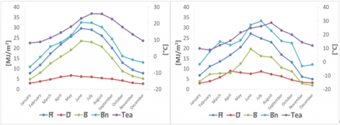
For the calculation of the energy produced, the global radiation on horizontal plane and the external air temperature, from historical climate data of Italian technical regulations UNI 10349 [13] were used. The standard provides the conventional monthly average daily values necessary for the design and verification of technical installations. Diffuse, beam and direct normal solar radiation were evaluated using the Liu–Jordan method [14]. In order to estimate the energy produced by solar photovoltaic systems we also considered climate data measured in the weather station at the Mechanical Engineering department at the University of Calabria. In Figure 3, the monthly average daily trends of global, direct, diffuse and direct normal solar radiation and external air temperature for Cosenza are shown.
Figure 3. Monthly average daily values of the external air temperature, of the horizontal global, direct and diffuse solar radiation and of the direct normal solar radiation. Historical data on the left. Experimental data on the right.
4.2 Siegel method
In the case of flat-plate photovoltaic, we adopted the simplified Siegel method [15] that provides an estimation of the monthly average daily efficiency η̅, which depends on the monthly average daily values of the external air temperature ₸ea and of the incident solar radiation E̅ (Eq. 1).
$\bar{\eta}=\eta_{R} \cdot\left[1-\beta_{R} \cdot\left(\overline{T_{e a}}-T_{R}\right)-\frac{\beta_{R} \cdot(\overline{\tau \alpha}) \cdot \bar{V}_{k} \cdot \bar{E}}{n \cdot U_{c}}\right]$ (1)
Where the over-bar denotes monthly average daily quantities; ηR is the efficiency at the reference temperature TR and at solar radiation of 1000 W/m2; βR is the temperature coefficient and depends mainly on the material properties, having value of about 0.0045 K-1 for crystalline silicon modules [16]; n is the number of hours per day, Uc is the overall thermal loss coefficient; Vk is a dimensionless function of quantities as the sunset angle, the monthly average daily clearness index, and the ratio of the monthly average daily total radiation on the array to that on a horizontal surface.
Such efficiency is used for the evaluation, by the Eq. 2, of monthly average daily electrical energy supplied by the photovoltaic field E̅e, starting from monthly average daily values of solar radiation on the inclined plane E̅, calculated by the method of Liu and Jordan [17].
$\bar{E}_{e}=A \cdot \bar{\eta} \cdot \eta_{B O S} \cdot \bar{E}$ (2)
Where ηBOS is the BOS (Balance of System) efficiency.
4.3 Software TRNSYS
The energy production of flat-plate PV was also analyzed by the TRNSYS simulation software. In the calculation software it is possible to conduct hourly evaluations which are therefore more detailed compared to the Siegel method. In particular, in addition to the hourly variability of climate data, the coefficient τα is changed every hour as a function of the inclination of the photovoltaic module and the position of the sun in the sky. The entire photovoltaic system has been simulated starting from the generation of climate data to the annual estimation of the electrical energy produced, through the calculation of the radiation incident on the inclined surfaces. We also compared the results obtained by the simulation software (TRNSYS) with those obtained through the simplified Siegel method.
Only TRNSYS software was used for the hourly electrical energy produced by the concentrating photovoltaic. In the software, a specific Type for concentrating photovoltaic panels is not available, therefore, it was necessary to use one related to flat-plate photovoltaic plants (Type 94) making appropriate changes and additions. Solar tracking has been simulated by setting an incident angle very close to zero, thus taking into account the accuracy of the tracking system. Direct normal solar radiation generated by the dedicated Type is changed to take into account the imperfect alignment between the normal on the plane and the solar rays. Subsequently, this component of solar radiation is given as an input to the photovoltaic Type, setting a value of diffuse solar radiation equal to zero at each temporal instant. To take into account the concentration ratio of the photovoltaic cell an equivalent area providing the same solar radiation concentrated in the focus of the Fresnel lenses was evaluated. The algorithm for the evaluation of the Incident Angle Modifier was disabled. The calculation of the efficiency was performed using direct normal solar radiation. Any optical losses were already accounted for in the reference efficiency from the data sheets. The actual performance of the system, in turn, will vary during the year according to different climatic conditions and on the basis of the variation coefficients of the electrical characteristics depending on the temperature of the external air.
The five-parameter model was used in dynamic simulations, which better allows a description of the current-voltage characteristic of modules, which must be different from crystalline silicon modules [18].
5.1 Flat-plate photovoltaic plants
5.1.1 Siegel method
Figure 4 shows the trend of the monthly electrical energy produced by the three flat-plate photovoltaic fields by applying the Siegel method starting from standard and the experimental climatic data. The highest installed power in the Cube Building photovoltaic field determines the greater production of electrical energy, with a maximum value of 60 MWh in August. It is followed by the Monaci and the Library photovoltaic fields with a peak value, respectively, of approximately 50 MWh and 20 MWh. The efficiency calculated with the two sets of climate data for the various installations are very close, as the external air temperature values are very close (see Figure 3); thus the lower values of global solar radiation on the horizontal plane measured experimentally lead to an underestimation of the monthly electrical energy produced by the three photovoltaic plants, compared to those obtained with the historical data.
Figure 4. Comparison of the monthly electrical energy produced from the three plants obtained using the data of the standard and the experimental data for the three plants.
The comparison shows that the experimental data mainly affect the values of the variables and slightly the qualitative result. The annual electrical energy produced, estimated with historical and experimental data, respectively, is about 215 MWh and 174 MWh for the Library plant, 537 MWh and 436 MWh for the Monaci plant, and 604 MWh and 490 MWh for the Cube Building plant. Lower values of experimental solar radiation lead to an underestimation of annual electrical energy produced of approximately 19%. The manufacturability, estimated with historical and experimental data, respectively, is 1597.17 kWh/kW and 1298.32 kWh/kW for the Library and Monaci plants, 1376.42 kWh/kW and 1117.93 kWh/kW for the Cube Building plant.
5.1.2 Software TRNSYS
The results obtained by the dynamic simulation software have been synthesized through the monthly average daily values in order to make a comparison with those obtained by the Siegel method.
Using climate data provided by standard, the values shown in Figure 5 were obtained. Figure 5 also shows the results obtained by the Siegel method.
Figure 5. Comparison between the monthly electrical energy produced by three photovoltaic fields calculated by the Siegel method and by the TRNSYS dynamic software. Historical climatic data.
The trends show that the simplified Siegel method accurately predicts the production of electrical energy and provides values that are slightly lower in summer and slightly higher in winter. The greatest differences occur in July, for the summer period, and in January, for the winter one, and are due to the variability of the loss coefficient Uc that is considered constant in the Siegel method while the hourly values are calculated in the TRNSYS software. In fact, in these months there is a higher deviation of solar radiation and of the external air temperature compared to the standard reference values. In addition to this hourly variability in the TRNSYS software, also the coefficient (τα) changes.
The results of dynamic simulations using experimental climate data, synthesized through the monthly average daily values and compared with the results of the application of the Siegel method, are shown in Figure 6.
Figure 6. Comparison between the monthly electrical energy produced by the three solar photovoltaics calculated by the Siegel method and by the dynamic software TRNSYS. Experimental climatic data.
The comparison of the electrical energy produced by the three photovoltaic plants with the simplified procedure and the dynamic simulation procedure highlights the good estimation obtained by the Siegel method. In addition, in this case the slight differences are due to the variability of hourly climate data, the loss coefficient Uc and the coefficient τα.
Even with the dynamic simulation code values less than approximately 19% are obtained by using the experimental data compared with historical data.
The comparison between the Siegel method and TRNSYS software results, referring to both historical data and to experimental data, showed that the simplified method accurately predicts the performance of a photovoltaic plant with deviations that remained around 4-5% in all cases.
5.2 Concentrating photovoltaic plant
The hourly electrical energy produced by concentrating photovoltaic fields is calculated solely by the software TRNSYS, as the simplified Siegel method cannot be used. The monthly average daily values were assessed after averaging the daily values for each month of the year.
The results obtained by means of the dynamic simulation software starting from historical and experimental data are shown in Figure 7 in terms of monthly electrical energy. In particular, an annual energy production respectively of 1128 MWh and 1133 MWh is obtained using the historical and experimental data. In the two cases, manufacturability results as being 2386.6 kWh/kW and 2398.9 kWh/kW.
Figure 7. Monthly electricity produced by concentrating photovoltaic using standard and experimental data.
5.3 Total electrical energy produced by the plants
Figure 8 shows the total electrical energy that can be produced by photovoltaic plants considering both experimental and historical climate data.
Figure 8. Monthly total electrical energy of the photovoltaic fields obtained with the historical and experimental climatic data.
The figure shows that the climate data markedly influences the estimation of electrical energy. The simplified calculation method of Siegel allows the making of very accurate assessments, in which in summer the results are close to the results generated by the dynamic procedure, while in winter the difference is slight. The results also showed that estimation by the Siegel method lead an error of about 3%, regardless of the climate data used. The latter however, regardless of the calculation method used, have significant influence obtaining a variance percentage of about 10%.
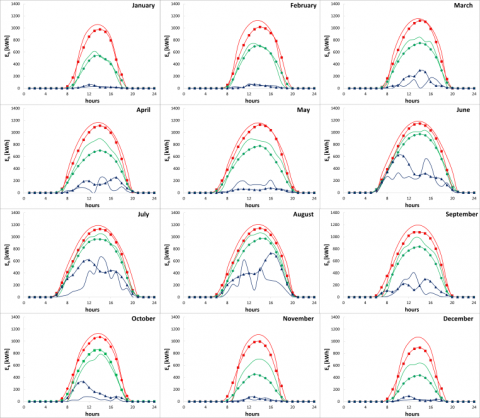
The method based on the monthly average day has the advantage of requiring few input data, represented by a value of each quantity for each month of the year. Such a simplified method, however, does not allow for knowledge of evolution in time, for example on an hourly basis, of electrical energy produced, so as to be able to identify the days and hours with the maximum and minimum production. The results obtained by the TRNSYS software, based on the both experimental and historical data, have been summarized by the monthly average hourly values, and hourly trends of days that experience the highest and the lowest production of electrical energy for each month of the year.
Figure 9 highlights the differences between the results obtained by means of historical data and experimental data.
Figure 9. Comparison of monthly average hourly values and hourly values of the days that are experiencing the highest and lowest total electrical energy produced for each month of the year obtained using historical and experimental data.
The difference is especially significant above all on the monthly average hourly trend. Instead, in the days when maximum production occurs, the trends are very close.
The electricity produced on an hourly basis shows a maximum between the hours 12:00 and 14:00 and becomes null at night, at different times depending on the month. This is due to the change in time, during the year in which sunrise and sunset occur. The maximum hourly energy produced during the year is around 1000 kWh and has variations limited in the various months. However, the monthly average hourly values are highly variable and present values close to those of the hourly trend of the day with maximum energy production in the summer months and are further from them in winter. This leads to increased production in the summer season.
5.4 Self-consumed and auxiliary energy
The monthly average daily values of the electrical energy needs and of the electrical energy produced and self-consumed, calculated by the Siegel method, were used for evaluating the monthly average daily energy need to be integrated through a transfer from the electrical national grid, as reported in Table 2.
Table 2. Monthly electrical energy consumption, self-consumed, and auxiliary electrical energy.
|
Consumption |
Self-consumed |
Auxiliary |
|
|
kWh |
kWh |
kWh |
|
|
January |
1631860 |
118837 |
1513023 |
|
February |
1516564 |
147531 |
1369033 |
|
March |
1575010 |
209689 |
1365321 |
|
April |
1289752 |
219288 |
1070464 |
|
May |
1374852 |
248799 |
1126053 |
|
June |
1639296 |
280992 |
1358304 |
|
July |
2107476 |
292518 |
1814958 |
|
August |
1337476 |
283412 |
1054064 |
|
September |
1530992 |
233370 |
1297622 |
|
October |
1334284 |
170911 |
1163373 |
|
November |
1436620 |
144166 |
1292453 |
|
December |
1522800 |
133764 |
1389036 |
|
Total |
18296982 |
2483279 |
15813703 |
|
% consump. |
13.57 |
86.43 |
Of the annual demand of electrical energy, equal to about 18.3 GWh, approximately 13.6% or 2.5 GWh are covered by the use of solar energy, while the rest of 15.8 GWh is to be integrated. In addition, it can be seen in any month that the electrical energy produced is completely self-consumed by users, as it is always less than the electrical energy need. The percentage of the total electrical energy consumption covered by the production of Library, Monaci and Cube Building plants are, respectively, 1.17%, 2.93% and 3.30%. The highest percentage derives from the Botanic Garden concentrating plant, which alone, through energy self-consumed, is able to cover approximately 6% of total electricity needs.
The same analysis was also performed using hourly values of electrical energy consumption of users and the total electrical energy produced by the photovoltaic arrays. The hours in which the energy produced is higher than that required by the users are negligible compared to the 8760 hours that constitute the entire year. For this reason, the results in terms of annual electricity self-consumed totaled to 13.2%, against 13.6% obtained by using monthly data.
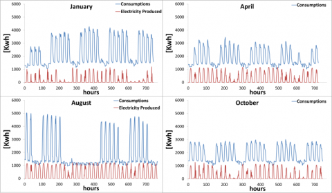
Figure 10. Hourly electrical energy produced and hourly consumption in four characteristic months of the year
It is necessary to highlight that the power of the photovoltaic fields is small if compared with the total contractual electrical power, with the specific purpose of maximizing self-consumption, as shown in Figure 10 representative of four months characteristic of the year. In any case, an analysis on an hourly basis allows for the self-consumed energy not to be overestimated, consequently allowing for the elimination of the portion of energy that is overproduced during peak hours, especially in summer.
The installation of a photovoltaic system involves an initial investment that is paid off over the years, in case of the absence of incentive mechanisms, as a result of the self-consumed part of the electrical energy produced. This type of intervention is capable of producing important economic returns especially in the case of large plants, such as the one analyzed in the present work. The analysis of the economic savings achievable as a result of the installation of photovoltaic plants at the University of Calabria is based on the estimated amount of self-consumed energy. Depending on the type of supply and the information derived directly from bills, the unit cost of electrical energy was obtained. In particular, it was noted that the cost of electricity supply is the sum of six components: generation, losses, dispatching, transport, tax revenue and increases (see Table 3).
Table 3. Cost components of the electricity supply.
|
GENERATION |
TRANSPORT |
||||
|
Band |
€/kWh |
Rate |
€/kWh |
||
|
F1 |
0.09091 |
Energy quote active |
0.00048 |
||
|
F2 |
0.08771 |
TRAS Component |
0.00568 |
||
|
F3 |
0.06851 |
|
|||
|
DISPATCH |
|||||
|
Rate |
€/kWh |
||||
|
Art. 44-44bis-45 del. AEEG 111/06 |
0.007072 |
||||
|
Component CD – art.48 AEEG del.111/06 |
0.000487 |
||||
|
Component INT – art.73.3 AEEG del.111/06 |
0.002102 |
||||
|
Component DIS – art.46 AEEG del.111/06 |
0.000615 |
||||
|
Componente RST – art.25 bis AEEG del.111/06 |
0.00045 |
||||
|
INCREASE |
|||||
|
Rate |
€/kWh |
||||
|
Components A-UC-MCT |
0.05226 |
||||
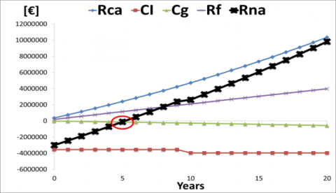
The losses were estimated as a percentage of self-consumed energy that, based on the information available from bills, is equal to 4%. For each hour of the year, the value of self-consumed energy and of the corresponding losses was calculated; so multiplying by the cost of the energy of the corresponding band, the value in euro, associated with the cost savings resulting from self-consumption of the energy produced by the photovoltaic plant at any hour of the entire year was obtained. To such annual cost saving, economic value of the components that are independent of the consumption band was added. Such components are due to dispatching, which was calculated by reference to the annual value of energy saved (self-consumption plus losses), transportation and increases, calculated with reference to the annual value of self-consumed energy. To quantify the return on investment, the method of net present saving RNa was employed. The net present saving method provides an indication of the income produced by investment of energy saving after recovering the initial investment. RNa is equal to RNa=Rca-CI-Cg+Rf, where Rca is the term relating to cost savings added to the benefits, CI is the term for the costs of the investment, Cg is the cost of management and Rf are the tax savings. The annual average inflation rate was assumed to be 1.2 % [19], the rate of increase of the cost of electricity equal to 0.029 [20], the discount rate equal to 0.003 [21] and the rate of increase in maintenance costs amounts to 0.12. The cost of initial investment is the sum of the cost of the three plants, equal to 3,627,162 €. Furthermore, it has been assumed that the replacement of the inverters in all systems takes place in the tenth year, with a cost of 3,543,528 €. It is assumed that the entire investment is made with equity and that there are no revenues from the sale of electrical energy. The values in Table 3, distinct per band and obtained from bills, were used for the electrical energy costs. Moreover, as regulated by AEEGSI 609/2014/R/EEL and 675/2014/R/COM resolutions, and successive modifications, for simple systems of production and consumption that obtain the qualification of SEU (Efficient Systems of User), it is necessary to consider an increase computed on the produced and self-consumed energy. The increase is equal to P x Hours x α x Rate, where P is the power plant expressed in kWp, Hours=1200, α = 0.35 for solar energy and Rate = 0.273 c€/kWh. After the installation of photovoltaic plants, the annual cost of electrical energy is linked to the difference between consumption and the energy produced by the plants, or rather the auxiliary energy required, to be drawn from the national electrical grid. The cost of electricity after the investment amounted to 2,563,910 € with an annual saving of 377,477 €. Applying the RNA method to the results obtained with the TRNSYS simulation software, a payback period slightly higher than the fifth year is obtained. The value of RNA at the end of the period of analysis is 9,829,887 €. Figure 11 shows the trend of the cumulative of the various terms that constitute RNa: Rca, CI, Cg and Rf.
Figure 11. Cumulative RNA and its cumulative terms
Cumulative curve of CI, term relative to investment costs, remains constant until the tenth year in which it undergoes a slight decrease due to the replacement cost of the inverters, which according to common practice, are supposed to have a useful life of ten years. Consequently, the cumulative curve of RNA undergoes a slight lowering then growing again until the twentieth year. The benefit/cost ratio [22] is equal to 3.47, while the internal rate of return RI [22] amounted to 0.185 proving the goodness of the investment.
The use of renewable energy sources, from an environmental point of view, has the great advantage of reducing emissions of air pollutants and greenhouse gases. The environmental benefits obtained from the adoption of photovoltaic systems are proportional to the amount of energy produced, assuming that this will replace the energy otherwise provided by conventional fossil sources. The use of a photovoltaic plant involves a reduction of emissions and polluting substances into the atmosphere, which contribute to the greenhouse effect. With the decision EEN 3/08 n. 100/08, the Italian Regulatory Authority for Electricity Gas and Water AEEGSI [20], has fixed the value of the conversion factor for primary energy into electrical energy at 0.187 x 10⁻³ TEP/kWh (Equivalent Tons of Petroleum per year), while the environmental report ENEL [23] contains the conversion factors for the evaluation of grams of CO2, SO2, NOx and dust particles avoided for every kWh produced by a photovoltaic plant. The amount of fossil fuel avoided is 464.37 TEP/year. The estimate of pollutant emissions avoided due to the installation of flat-plate and concentrating photovoltaic plants are shown in Table 4.
Table 4. Pollutant emissions avoided through the installation of flat-plate and concentrating photovoltaic plants.
|
|
CO2 |
SO2 |
NOx |
Dust |
|
|
[t/year] |
[kg/year] |
[kg/year] |
[kg/year] |
|
Library |
185.04 |
97.03 |
128.80 |
3.01 |
|
Monaci |
462.59 |
242.57 |
321.99 |
7.51 |
|
Cube Building |
52.91 |
273.15 |
362.58 |
8.46 |
|
Botanic Garden |
972.05 |
509.70 |
676.60 |
15.79 |
In this work, we studied the energy, economic and environmental advantages of the flat-plate and concentrating photovoltaic plants, which are expected to be realized at the University of Calabria. The project involves the installation of three flat-plate and a concentrating photovoltaic plants. An analysis of electrical energy consumption of the university users was presented. A high electricity demand in summer was shown due to the higher consumption due to the cooling plant. The daily peak of consumption in winter is approximately 70 MWh, between the February 14th and February 25th, while in summer it is about 85 MWh on June 25th with annual electricity needs of around 18.3 GWh.
The results showed that the electrical energy produced on a monthly basis estimated by the Siegel method is very accurate, showing a difference of less than 5% compared to the hourly values obtained with TRNSYS, regardless of the climate data used. The latter however, regardless of the method of calculation used, strongly influences the results with a deviation rate of 10% between the results obtained using experimental data and the results provided employing the historical data from the standard. Of the annual demand of electricity, equal to 18.3 GWh, the Siegel method provides produced and self-consumed energy of approximately 13.6%, equal to 2.5 GWh, while with TRNSYS, which conducts an hourly estimation, the self-consumed percentage resulted equal to 13.2%.
Subsequently, a detailed economic analysis was conducted based on the results obtained with the dynamic simulations, in terms of energy saved on an hourly basis, appropriately considering the various components that determine the cost per hour of electricity. From the results of the economic analysis, it was shown that the payback period is around five years with a value of RNA at the end of the analysis period equal to 9,829,887 €. The benefit/cost ratio amounts to 3.47 with an internal rate of return equal to 0.185.
Finally, an environmental analysis allowed for the estimation of the amount of fossil fuel and pollutant emissions avoided using photovoltaic technology.
|
a |
Modified ideality factor |
|
B |
Beam solar radiation on the horizontal plane [W/m2] |
|
Bn |
Direct normal solar radiation [W/m2] |
|
C |
Electricity consumption [J] |
|
CI |
Cost of the investment [€] |
|
Cg |
Cost of management [€] |
|
D |
Diffuse solar radiation on the horizontal plane [W/m2] |
|
E |
solar radiation incident on PV array [W/m2] |
|
Ee |
Electrical energy produced by the PV [J] |
|
H |
Global solar radiation on the horizontal plane [W/m2] |
|
I |
Current [A] |
|
IL |
Module photocurrent [A] |
|
I0 |
Diode reverse saturation current [A] |
|
Impp |
Current at maximum power point [A] |
|
ISC |
short-circuit current [A] |
|
NOCT |
Nominal Operating Cell Temperature [°C] |
|
Pp |
plant peak power [kWp] |
|
Pp,mod |
module peak power [W] |
|
Rca |
Cost savings added to the benefits [€] |
|
RI |
Internal rate of return [€] |
|
Rf |
Tax savings [€] |
|
RNa |
Net present savings [€] |
|
Rs |
series resistance [Ω] |
|
Rsh |
shunt resistance [Ω] |
|
TR |
Reference temperature [°C] |
|
₸ea |
External air temperature [°C] |
|
Uc |
Array thermal loss coefficient [W/(m2 K)] |
|
V |
Voltage [V] |
|
Vk |
Dimensionless function [-] |
|
Vmpp |
Voltage at maximum power point [V] |
|
VOC |
Open-circuit voltage [V] |
|
Greek symbols |
|
|
β |
Slope of PV array [°] |
|
βR |
Temperature coefficient [°] |
|
η |
Efficiency [-] |
|
ηR |
Efficiency at the reference temperature [-] |
|
ηBOS |
Efficiency of BOS (Balance of System) [-] |
|
τα |
Module transmittance-absorptance product [-] |
|
ΔISC |
Temperature coefficient of short-circuit current [%A/°C] |
|
ΔVOC |
Temperature coefficient of open-circuit voltage [%V/°C] |
|
Symbols |
|
|
– |
Monthly average daily value |
1. European commission, http://ec.europa.eu/europe2020/europe-2020-in-a-nutshell/targets/index_it.htm. Last access: November 2015.
2. Duffie J.A., Beckman W.A., Solar Engineering of Thermal Processes 4th Edition, Solar Energy Laboratory University of Wisconsin-Madison, John Wiley & Sons, 2013.
3. Pavel Y.V., Gonzalez H.J., Vorobiev Y.V., “Optimization of the solar energy collection in tracking and non-tracking PV solar system,” Proceedings of the 1st International Conference on Electrical and Electronics Engineering, ICEEE; 2004. pp.310–314. DOI: 10.1109/ICEEE.2004.1433900.
4. Mo S., Chen Z., Hu P., “Performance of a passively cooled Fresnel lens concentrating photovoltaic module,” IEEE Asia Pacific Power and Energy Engineering Conference, 2011. pp.1–4. DOI: 10.1109/APPEEC.2011.5747676.
5. Pérez-Higueras P.J., Rodrigo P., Fernández E.F., Almonacid F., Hontoria L.A., “A Simplified method for estimating direct normal solar irradiation from global horizontal irradiation useful for CPV applications,” Renewable and Sustainable Energy Reviews, 16 (2012) 5529–5534. DOI: 10.1016/j.rser.2012.05.041.
6. Bin Du, Eric Hu, “Mohan Kolhe, “Performance analysis of water cooled concentrated photovoltaic (CPV) system,” Renewable and Sustainable Energy Reviews, 16 (2012) 6732 – 6736. DOI: 10.1016/j.rser.2012.09.007.
7. Segev G., Kribus A., “Performance of CPV modules based on vertical multi-junction cells under non-uniform illumination,” Solar Energy, 88 (2013) 120–128. DOI: 10.1016/j.solener.2012.11.020.
8. Baig H., Sarmah N., Heasman K.C., Mallick T.K., “Numerical modelling and experimental validation of a low concentrating photovoltaic system,” Solar Energy Materials & Solar Cells, 113 (2013) 201–219. DOI: 10.1016/j.solmat.2013.01.035.
9. Yadav P., Tripathi B., Lokhande M., Kumar M., “Estimation of steady state and dynamic parameters of low concentration photovoltaic system,” Solar Energy Materials & Solar Cells, 112 (2013) 65–72. DOI: 10.1016/j.solmat.2013.01.012.
10.Cucumo M., Ferraro V., Marinelli V., Cucumo S., Cucumo D., “LCA analysis of a solar concentration system for the micro-Chp and comparison with a PV plant,” International Journal of Heat and Technology, 30 (1) (2012) 63-68. DOI: 10.18280/ijht.300110.
11.Oliveti G., Arcuri N., Bruno R., Girovasi D., “Energy characterization of an unglazed pv/t panel for the production of electricity, heating and cooling,” International Journal of Heat and Technology, 32(1-2) (2014) 219-24.
12. TRNSYS 17 - A TRaNsient System Simulation program - Volume 4, Mathematical Reference, 2010.
13. UNI 10349:1994, Heating and Cooling of Buildings, Climatic Data.
14. Liu B.Y.H., Jordan R.C., “The interrelationship and characteristic distribution of direct, diffuse and total solar radiation,” Solar Energy 4(3) (1960) 1-19. DOI: 10.1016/0038-092X(60)90062-1.
15. Siegel M.D., Klein S.A., Beckman W.A., “A simplified method for estimating the monthly-average performance of photovoltaic systems,” Solar Energy, 26 (1981) 413-8. DOI: 10.1016/0038-092X(81)90220-6.
16. Notton G., Cristofari C., Mattei M., Poggi P.P., “Modelling of a double-glass photovoltaic module using finite differences,” Applied Thermal Engineering, 25 (2005) 2854-77.
17. Liu B.Y.H., Jordan R.C., “Daily insolation on surfaces tilted towards the equator,” ASHRAE Journal, 3(10) (1961) 53-9.
18. Fry, Bryan, “Simulation of grid-tied building integrated photovoltaic systems,” M.S.Thesis – Solar Energy Laboratory, University of Wisconsin, Madison: 1999.
19. National Institute of Statistics ISTAT, http://www.istat.it/it/archivio/109705. Last access: November 2015.
20. Italian Regulatory Authority for Electricity Gas and Water AEEGSI, http://www.autorita.energia.it. Last access: November 2015.
21. EURO Inter Bank Offered Rate EURIBOR, http://www.euribor.it/tassi-storici-euribor. Last access: November 2015.
22. Cucumo M.A., Marinelli V., Oliveti G., “Ingegneria solare: principi ed applicazioni,” Pitagora Editrice Bologna, 1994.
23. Environmental Report 2013, National Entity for Electricity ENEL, www.enel.com. Last access: November 2015.