Maher Abd Ameer Kadim | Isam Issa Omran | Alaa Ali Salman Al-Taai*
© 2021 IIETA. This article is published by IIETA and is licensed under the CC BY 4.0 license (http://creativecommons.org/licenses/by/4.0/).
OPEN ACCESS
Flood forecasting and management are one of the most important strategies necessary for water resource and decision planners in combating flood problems. The Muskingum model is one of the most popular and widely used applications for the purpose of predicting flood routing. The particle swarm optimization (PSO) methodology was used to estimate the coefficients of the nonlinear Muskingum model in this study, comparing the results with the methods of genetic algorithm (GA), harmony search (HS), least-squares method (LSM), and Hook-Jeeves (HJ). The average monthly inflow for the Tigris River upstream at the Al-Mosul dam was selected as a case study for estimating the Muskingum model's parameters. The analytical and statistical results showed that the PSO method is the best application and corresponds to the results of the Muskingum model, followed by the genetic algorithm method, according to the following general descending sequence: PSO, GA, LSM, HJ, HS. The PSO method is characterized by its accurate results and does not require many assumptions and conditions for its application, which facilitates its use a lot in the subject of hydrology. Therefore, it is better to recommend further research in the use of this method in the implementation of future studies and applications.
flood routing, nonlinear Muskingum model, particle swarm optimization (PSO), genetic algorithm (GA), harmony search (HS), least-squares method (LSM), Hook-Jeeves (HJ)
Floods have catastrophic social and economic consequences for the environment [1, 2], including the destruction of dams [3], the inundation of residential and industrial areas, the disruption of transportation networks [4], the damage to crops, and the destruction of agricultural areas [5]. As a result, flood forecasting and control is a critical concern of water policy-makers and designers [6, 7]. Flood forecasts are made using hydrologic and hydraulic models. Flood routing is the process of estimating the downstream flood discharge hydrograph based on the upstream discharge hydrograph [8, 9]. Flood routing can be performed using hydraulic models based on numerical approaches, although it requires complex flow equations [10]. Hydrological models use the spatially aggregated continuity equation and storage equation to the routing of floods. These algorithms require only a small amount of data to predict floods [11]. The Muskingum Model is an outstanding hydrological model in flood management. This model has a number of parameters that must be obtained for accurate flood forecasting [12], and several versions of the model have been used to route flooding. The use of the optimization method is one of the options for calculating parameters as choice variables. The ability of evolutionary algorithms to solve optimization method problems is impressive. These algorithms are characterized by the adaptability, fast, and accuracy of their application [13]. As a result, evolutionary algorithms can be used to calculate those parameters [14]. A nonlinear Muskingum model with the lateral flow was used in flood routing [15].
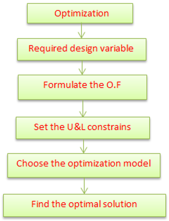
Some optimization techniques, such as genetic algorithm (GA) [16] and harmony search (HS) [17] were used to calibrate the three parameters of Muskingum's model which are K, x, and m. The least-squares method (LSM) was also used to determine the parameters of Muskingum's nonlinear model [18]. The Hook-Jeeves pattern (HJ) in combination with linear regression (LR), conjugate gradient (CG), and David-Fletcher-Powell (DFP) applications were also used to estimate these parameters [19, 20]. When comparing the performance of the method with the Gill's procedure, it was observed that HJ + CG and HJ + DFP gave better results. When most actual river systems have a nonlinear relationship between storage and discharge, the linear model may be inappropriate. All the previous methods do not represent the best method, and they may be limited and trapped at a certain point. The parameters of the model were estimated using GA [16]. The results revealed that the GA estimate was superior to earlier approaches and that the initial guess did not have to be close to the optimum. The HS was used to solve a similar problem [21, 22]. Their findings revealed that the HS estimate outperformed GA and did not necessitate an initial guess that was near to the optimum. In this study, the particle swarm optimization (PSO) [23, 24] methodology is used to estimate the parameters of the nonlinear Muskingum model in this study, then the results compared with GA, HS, LSM, and HJ. Also, the results were also confirmed by performing statistical analysis of three types of error measurement indices (SSD, ETP, and MARE) [25] used to evaluate the performance of each algorithm. Simulation results indicate that the proposed scheme can improve the accuracy of the Muskingum model for flood routing. Figure 1 shows the steps of the optimal design procedure.
Figure 1. Steps of the optimal design procedure [19]
Considering the excellent performance of SOS in exploitation stage and the strong ability of other algorithms in exploring the solution space, we attempt to combine the advantages of these algorithms together. Moreover, the practical swarm is also taken into consideration to improve the efficiency.
The nonlinear storage and continuity equations presented below are often used in applications of the Muskingum model:
$\frac{d S}{d t}=I-Q$ (1)
$S=K[X I+(1-X) Q]$ (2)
The rate of outflow can be written as follows:
Qi = {1/1-x} {Si/k}m-1 - {x/1-x}Ii (3)
From Eq. (1) and (3), the results of combination:
Qi = {1/1-x} {Si/k}m-1 + {1/1-x}Ii (4)
Si+1= Si +∆Si (5)
Qi+1 = {1/1-x} {Si+1/k}m-1- {x/1-x}I-i +1 (6)
where: I-i+1 = (Ii+1+Ii)/2.
The steps of the routing procedure are as follows [14, 18]:
Suppose values for the three parameters: K, X, and m.
Use Eq. (2) to calculate storage (S) when the initial outflow equals the initial inflow.
Use Eq. (4) to calculate the time rate of storage volume change.
Use Eq. (5) to calculate the following accumulated storage.
Eq. (6) is used to determine the next outflow.
(I-t+1) indicates the average inflow (It+1+It /2). When the storage ratio (t/t+1) is greater than 2, it is replaced by (It+1+It /2).
3.1 Particle Swarm Optimization (PSO)
The PSO is used to estimate parameters for the nonlinear Muskingum model in this study. Particles in a PSO system move around in a multidimensional search space. During the movement, each particle adjusts its position based on its own experience and the experience of a neighboring particle, utilizing the best position encountered by itself and its neighbor [23, 24, 26, 27].
The Objective function is written as follows: A current ith particle position in the multidimensional search space that represents Yin at the nth iteration, a current's speed Vin is in charge of the movement's speed and direction. In Eq. (7), each particle's velocity update along each dimension to the local and global best positions, and in Eq. (8), each particle's position update [28].
Vin+1=Vin + c1r1(Pi-yi) + c2r2(Pj – yin) (7)
Yin+1=yi + Vin+1 (8)
where:
Pi: the particle's best previous position.
Pj: The particle with the best global position out of all the particles.
c1 and c2 are acceleration parameters that each control how far the particle moves within a single iteration.
r1 and r2 are coefficients taken from two uniform random numbers within the limits from 0 to 1.
Eq. (9) and Eq. (10) are used to update and apply the best local values in the field.
$\begin{aligned} \mathrm{Pi} &=\{\mathrm{Pi}: \mathrm{f}(\mathrm{yi}) \geq \mathrm{f}(\mathrm{Pi})\\ \mathrm{Pi} &=\{\mathrm{Pi}: \mathrm{f}(\mathrm{yi})<\mathrm{f}(\mathrm{Pi})\end{aligned}\}$ (9)
Or
Pj = min.[f(Pi)] i= 1,2,3,……..,m (10)
where: m is the total number of particles and f is the objective function.
3.2 Genetic Algorithm (GA)
In recent years, a slew of optimization strategies has evolved that use random search algorithms to simulate natural evolutionary processes. This type of approach could be utilized to solve optimization problems that aren't well suited to deterministic methods. Algorithms for problems with discontinuous non-differentiable, stochastic, or extremely nonlinear objective functions are included, and Genetic Algorithms are some of the algorithms that fall into this category [16, 29]. The first stage in a GA is to establish a random population, with each person having a unique fitness. A chromosome is a collection of genes that is coded in string form for each individual.
To provide a description of an individual in the population of interest, chromosome representation is required. After each chromosome has been decoded, the performance function is utilized to assess its fitness. Individuals who are more physically fit will be able to make a greater contribution to future generations [30]. Figure 2 shows the flowchart of GA.
Figure 2. Flowchart of the Genetic Algorithm (GA) [30]
The decoded value is obtained as follows [30]:
Xdec= Xmin + Xbi (Xmax.- Xmin.)/2n-1 (11)
The fitness value of each individual is determined by the following:
F(xj) = 2 – P2 + {2(PZ-1)XJ}/m-1 (12)
3.3 Harmony Search (HS) Algorithm
The Harmony Search (HS) algorithm is a form of optimization in a variety of water resources engineering challenges as an optimization methodology, the following relation is the definition of the objective function [17, 21, 22]:
Min. Z(X) Subject to xJ ϵ XJ ; XJL≤ ҲJ ≤ XJU (13)
where:
(J =1,2, …., N).
Z(X): the objective function.
XJ: design variable.
ҲJ: is the set of all possible values for each decision variable.
xiL and xiU are the decision variable lower and upper bounds.
N is the number of design variables.
Figure 3 shows a flow chart of the procedure employed in operations. The method's major components are: collecting the relevant data (land use, river cross-section, inflows), and utilizing the HS algorithm to optimize the procedure.
Figure 3. Flowchart of the harmony search algorithm (HS) [21, 22]
3.4 Analytical procedures for regression analysis
The researchers used multiple linear regression analysis to demonstrate the hydrological factors that best explain flood flow changes and to construct equations to predict flood flows. Figure 4 shows a flowchart of the regression analysis. In most cases, the regression equation is expressed as [12, 31]:
$\mathrm{y}=\mathrm{a}_{0}+\sum_{i=1}^{m} ai. x i+\sum_{i=1}^{m} aii. x^{2}+\sum_{i=1}^{m} \sum_{i=1}^{m} { aij.xi.xj }+\varepsilon$ (14)
where:
Y: the variable of response;
X: factors of explanatory;
a: regression coefficients.
Figure 4. Flowchart of the multiple linear regression analysis [12, 31]
3.5 Hooks-Jeeves pattern search model (HJ)
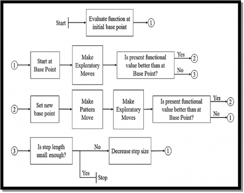
The pattern search approach iteratively generates a collection of search directions. The search directions should be established in such a way that they totally cover the search space. This necessitates at least N linearly distinct search directions in an N-dimensional issue. In a two-variable function, for example, it requires at least two search directions to move from one place to another. It is noticed that some groups of N search directions can reach the target faster (need a few iterations), while others may need more iterations. A mixture of exploratory moves and heuristic pattern moves is done iteratively in the Hooke-Jeeves approach. To locate the optimal point surrounding the present position, an exploratory move is made in the area of the present position in a methodical manner, Figure 5 shows the pattern move for the unidirectional approach [16, 17].
Figure 5. Pattern move for the unidirectional approach [16, 17]
3.5.1 Exploratory step
Assume that (xc) represents the current solution (the starting point), assume that (A) has a negative impact on the variable (x percent); let j = 1 as well as x = xc.
1. Estimate
f = f (x), f + = f (xj + Δj) and f - = f (xj - Δj) (15)
2. Determine f min = min (f, f +, f -). Set x corresponds to f min.
3. Is j= N? If No: set j = j+ 1 and move to Step 1, or Yes: x becomes the required result and moves to Step 4.
4. Repeat the successful moves, assume the new point as the new base point if it has a higher fitness, whatever happens, go back to step 2.
5. Step length should be adjusted to the next smaller step. Continue from step 2 if there is a smaller step, otherwise, terminate.
The current point is disturbed in positive and negative directions along with each variable one at a time throughout the exploratory motion, and the best point is recorded. At the conclusion of each variable perturbation, the current point is changed to the best point. In any instance, the result of the exploratory maneuvers is deemed to be the best spot [16, 17].
3.5.2 Pattern move
Different A new point is discovered by leaping from the current best point xc in the direction of the previous best point a ‘1' and the current base point x(k), as follows:
Xp (m+1) = x (m) + (x(m) - x(m-1)) (16)
An iterative application of an exploratory move in the vicinity of the current location and a subsequent move using the pattern move make up the Hooke-Jeeves approach. The pattern move is not accepted if it does not take the solution to a better region, and the scope of the exploratory search is reduced [19, 20].
Figure 6 shows the flowchart for Hooks-Jeeves direct search, Table 1, indicate the complete algorithm of this model.
Table 1. The complete algorithm of the Hooks-Jeeves pattern search model (HJ)
|
Algorithmic Framework |
Hooke-Jeeves Pattern Search Algorithm |
Dimensional Local Search Algorithm |
|
1. Set the coordinates of the starting base point xt to be uniformly random. To construct a set of candidates, search the space in even intervals in each dimension. As the local search's foundation, choose the best candidate xt+1.
2. Use one of the local search alternatives described in sections A and B to find anything nearby. Save the locally optimized solution xt+n if it isn't within a certain distance of any other solution.
3 Steps 1 and 2 should be repeated as long as the objective function remains the same.
4. Reoptimize the stored solutions when a change occurs by using the appropriate local search. |
1. Obtain the xt starting base point. Set a range of step lengths.
2. At a time, move the base point along each of the d dimensional axes. time and assess the outcome Adopt each new point if it improves on the previous one. the preceding point Proceed to step 3 if any of the movements were successful. If there are none, was successful, go on to number four.
3. In a combined pattern move, repeat the successful moves. Assume the new point as the new base point if it has a higher fitness. Whatever happens, go back to step 2.
4. Step length should be adjusted to the next smaller step. If there's a smaller step, take it. continue from the second. If this is not the case, the process should be ended. |
1. Obtain the xt starting base point. Set a range of step lengths.
2. Sequence through the dimensions by moving the base point along one of the d dimensional axes at a time. Examine the outcome. Adopt the new coordinates and repeat in the next dimension if the fitness is better than the prior solution.
3. Change the step length. If there are no further steps, end the process. If there are further stages, go to step 2.
|
Figure 6. Flowchart of the Hooks-Jeeves pattern search model (HJ) [19, 20]
3.6 Statistical analysis, error measurement indices
In this study, the index sum of squared deviations (SSD) was used as the objective function. The total discrepancies between observed and actual discharges are calculated by using the following equation [7, 8, 25]:
Min. $\mathrm{SSD}=\sum_{i=1}^{m}|Q o b o-Q e s o|$ (17)
where:
Qobo = observed outflow (m3/s);
Qeso = simulated outflow (m3/s).
ETP (Error of Time to Peak): The ETP index calculates the difference between projected and observed discharge time discrepancies:
ETP = (TPO – TPC) (18)
where:
TPO = time peak of observed outflow hydrograph;
TPC = time peak of routed outflow hydrograph.
The mean of the relative error between observed and routed outflows is called the mean absolute relative error (MARE):
MARE $=\frac{1}{m} \sum_{j=1}^{m} \frac{\mid Q o b s .-Q rou. \mid}{Q o b s .}$ (19)
where:
Qobs. = observed outflow;
Qrou. = routed outflow;
m= number of data.
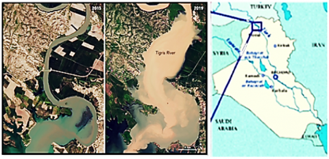
The length of the Tigris River is 1,750 km, and it starts from the Taurus Mountains in eastern Turkey, about 25 km southeast of Elazig and about 30 km from the headwaters of the Euphrates River. The river then passes through southeastern Turkey for a distance of 400 km until it reaches the Syrian-Turkish border. The only part of the river that runs through Syria is 44 km long. The Tigris River enters the Iraqi territory from the north, and its flow continues towards the south of the country, and during the distance of flow of more than 1,200 km, a number of tributaries coming from Iranian lands pour into it. The main channel of the river continues south until the Tigris River joins the Euphrates River in the Qurna region to form the Shatt al-Arab. The region of the Tigris River, located at its entrance from the northern region of the country, and the extension of its course to the upstream course of the Mosul Dam, was selected as a case study. This area has regular hydrological and hydrological characteristics, in addition to the absence of major tributaries entering or leaving the river [32]. Figure 7 shows the layout of the study area.
Figure 7. Layout of the study area [32]
It is difficult to estimate the nonlinear Muskingum model parameters through trial and error. Various approaches have been used to estimate these parameters throughout the last two decades. One of the strategies that have been successful in estimating these parameters is optimization approaches. The PSO method was utilized to estimate the three parameters of the nonlinear Muskingum model in this study. The performance of the PSO method was evaluated by comparing the results of its implementation with the results of applying different heuristic algorithms such as GA, HJ, LSM, HS, and exploring who is the best to find the optimal values of Muskingum's nonlinear parameters in guiding floods. The statistical indicators SSD, ETP, and MARE have been used to evaluate previous applications.
The analytical results shown in Table 2 for the comparison between the observed values and the routed outflow values, as well as the results of the statistical analysis presented in Table 3, showed that the results of the PSO method were the best, and the closest to the observed results, and this is what was observed in Figure 8. The descending sequence of the efficiency evaluation rate of the optimization methods in terms of their compatibility with the observed results was as follows: PSO, GA, LSM, HJ, and HS, according to the computed error index value for each method.
Table 4 shows the values of Muskingum's nonlinear coefficients calculated using the optimization methods adopted in this study, where it was noted that the use of the PSO method is the best in calculating these coefficients compared to the results of other methods, and also in terms of their compatibility with the results of the Muskingum model. The descending sequence of the efficiency evaluation rate of the optimization methods was as follows: PSO, GA, LSM, HJ, HS.
Table 2. Observed and routed outflow for various methods
|
Time (hr.) |
Inflow (cms) |
Observed Outflow (cms) |
Routed Outflow (cms) |
||||
|
PSO |
GA |
HS |
LSM |
HJ |
|||
|
0 |
144 |
122 |
112.0 |
131.0 |
130.8 |
126.9 |
131.0 |
|
6 |
141 |
155 |
150.8 |
162.0 |
160.8 |
146.0 |
159.0 |
|
12 |
204 |
210 |
189.3 |
221.5 |
230.7 |
217.0 |
214.0 |
|
18 |
190 |
210 |
187.5 |
219.0 |
243.0 |
217.0 |
205.0 |
|
24 |
192 |
214 |
190.0 |
223.0 |
232.7 |
220.6 |
217.0 |
|
30 |
186 |
190 |
210.0 |
205.0 |
220.0 |
211.0 |
202.0 |
|
36 |
170 |
177 |
188.6 |
187.0 |
190.0 |
180.4 |
180.5 |
|
42 |
165 |
206 |
211.0 |
218.0 |
220.7 |
210.7 |
210.6 |
|
48 |
135 |
160 |
176.0 |
178.0 |
190.6 |
171.0 |
168.0 |
|
54 |
188 |
220 |
223.0 |
201.0 |
254.6 |
211.0 |
223.0 |
|
60 |
254 |
210 |
221.4 |
219.0 |
232.0 |
216.0 |
215.0 |
|
66 |
430 |
400 |
410.0 |
421.0 |
433.6 |
411.0 |
412.0 |
|
72 |
705 |
710 |
700.9 |
718.0 |
732.8 |
700.8 |
720.0 |
|
78 |
1010 |
720 |
712.0 |
716.0 |
741.0 |
705.0 |
731.0 |
|
84 |
1190 |
755 |
733.2 |
740.8 |
720.0 |
751.0 |
760.0 |
|
90 |
700 |
700 |
700.0 |
721.0 |
732.0 |
709.0 |
703.0 |
|
96 |
410 |
720 |
719.7 |
712.0 |
741.7 |
714.0 |
717.0 |
|
102 |
220 |
750 |
730.0 |
870.0 |
763.0 |
755.0 |
745.0 |
|
108 |
210 |
890 |
880.2 |
865.0 |
870.0 |
885.0 |
884.9 |
|
114 |
189 |
880 |
895.0 |
854.8 |
840.0 |
840.0 |
879.0 |
|
120 |
156 |
510 |
512.0 |
541.0 |
540.2 |
501.0 |
503.0 |
|
126 |
150 |
290 |
287.9 |
220.0 |
310.0 |
280.0 |
203.3 |
|
132 |
135 |
210 |
201.0 |
218.0 |
221.0 |
206.8 |
211.0 |
|
138 |
144 |
190 |
194.0 |
188.6 |
210.0 |
185.7 |
185.0 |
|
144 |
110 |
180 |
190.0 |
185.5 |
202.7 |
179.0 |
175.0 |
|
150 |
95 |
154 |
161.0 |
154.7 |
160.0 |
154.5 |
150.0 |
|
156 |
88 |
130 |
127.0 |
131.0 |
143.0 |
132.0 |
132.0 |
|
162 |
80 |
120 |
121.0 |
124.0 |
136.0 |
123.0 |
116.0 |
|
168 |
77 |
115 |
117.9 |
118.0 |
125.0 |
113.0 |
112.0 |
|
174 |
70 |
110 |
116.0 |
114.0 |
122.0 |
112.0 |
107.0 |
|
180 |
65 |
112 |
115.0 |
116.0 |
123.0 |
115.0 |
110.5 |
|
186 |
60 |
110 |
112.0 |
113.0 |
122.0 |
116.0 |
106.0 |
|
192 |
55 |
104 |
106.0 |
102.0 |
121.0 |
102.0 |
100.0 |
|
198 |
50 |
100 |
101.0 |
103.0 |
112.0 |
102.0 |
98.6 |
Table 3. Computed error index value for each method
|
Statistical method |
PSO |
GA |
HS |
LSM |
HJ |
|
SSD |
3122150 |
3155210 |
3564512 |
3136561 |
3463312 |
|
ETP |
1 |
2 |
5 |
2 |
3 |
|
MARE |
0.060 |
0.084 |
0.360 |
0.086 |
0.284 |
Table 4. Computed nonlinear Muskingum parameters
|
Muskingum parameters |
Muskingum |
PSO |
GA |
HS |
LSM |
HJ |
|
K |
0.191 |
0.190 |
0.180 |
0.070 |
0.175 |
0.091 |
|
X |
0.352 |
0.350 |
0.311 |
0.270 |
0.321 |
0.310 |
|
m |
2.153 |
2.131 |
1.990 |
2.560 |
2.330 |
2.540 |
Figure 8. Simulated outflow hydrograph for Tigris River
By analyzing the results of the general evaluation process for the efficiency of the optimization methods and comparing them with the results of applying the Muskingum model, it can be said that the Particle Swarm Optimization (PSO) method is the best, followed by the Genetic Algorithm (GA) method, and then the rest of the other improvement methods.
In this study, different optimization methods were used in calculating and analyzing the results of the routed outflow within the study area in the Tigris River and comparing them with the results of applying the Muskingum model and calculating its parameters.
The analytical and statistical results showed that the PSO method is the best application and corresponds to the results of the Muskingum model, followed by the GA method, according to the following general descending sequence: PSO, GA, LSM, HJ, HS.
The advantage of the PSO method over other optimization methods is not only in its accurate results but also in the requirements for its application since it does not require many assumptions and conditions. From the above, it appears that the PSO method has a lot of potential in the topic of hydrology, which we recommend further research and implementation of future applications and studies.
Due to its excellent accuracy and simplicity, the Muskingum model is a valuable and essential hydrological model. Hydrological models can be completed after calculating parameter values; however, hydraulic models are necessary to simulate complicated boundary hydraulic conditions, which increases computing time. PSO has the benefit of not requiring the starting values of the model parameters to be assumed. The findings show that PSO can estimate the three parameters with a high degree of accuracy, resulting in accurate outflow forecasts. As a result, the model is also capable of anticipating outflow. No derivative is necessary with the PSO technique. PSO looks to have a lot of potential in the subject of hydrology, and further applications should be investigated.
[1] Bagatur, T., Onen, F. (2018). Development of predictive model for flood routing using genetic expression programming. Journal of Flood Risk Management, 11(2): S444-54. http://dx.doi.org/10.1111/jfr3.12232
[2] El-Shafie, A., Noureldin, A., Taha, M., Hussain, A., Mukhlisin, M. (2012). Dynamic versus static neural network model for rainfall forecasting at Klang River Basin, Malaysia. Hydrology and Earth System Sciences, 16(4): 1151-69. http://dx.doi.org/10.5194/hessd-8-6489-2011
[3] Mazzoleni, M., Noh, S.J., Lee, H., Liu, Y., Seo, D.J., Amaranto, A., Alfonso, L., Solomatine, D.P. (2018). Real-time assimilation of streamflow observations into a hydrological routing model: Effects of model structures and updating methods. Hydrological Sciences Journal, 63(3): 386-407. https://doi.org/10.1080/02626667.2018.1430898
[4] Zhou, Y., Guo, S., Chang, F.J., Liu, P., Chen, A.B. (2018). Methodology that improves water utilization and hydropower generation without increasing flood risk in mega cascade reservoirs. Energy, 143: 785-96. https://doi.org/10.1016/j.energy.2017.11.035
[5] El-Shafie, A., Mukhlisin, M., Najah, A.A., Taha, M.R. (2011). Performance of artificial neural network and regression techniques for rainfall-runoff prediction. International Journal of Physical Sciences, 6(8): 1997-2003. https://doi.org/10.5897/IJPS11.314
[6] Vatankhah, A.R. (2018). Discussion of “assessment of modified honey bee mating optimization for parameter estimation of nonlinear muskingum models” by Majid Niazkar and Seied Hosein Afzali. Journal of Hydrologic Engineering, 23(4): 7018002. https://doi.org/10.1061/(ASCE)HE.1943-5584.0001603
[7] Yaseen, Z.M., Fu, M., Wang, C., Mohtar, W.H.M.W., Deo, R.C., El-Shafie, A. (2018). Application of the hybrid artificial neural network coupled with rolling mechanism and grey model algorithms for streamflow forecasting over multiple time horizons. Water Resources Management, 32(5): 1883-99. https://doi.org/10.1007/s11269-018-1909-5
[8] Elzwayie, A., El-Shafie, A., Yaseen, Z.M., Afan, H.A., Allawi, M.F. (2017). RBFNN-based model for heavy metal prediction for different climatic and pollution conditions. Neural Computing and Applications, 28(8): 1991-2003. https://doi.org/10.1007/s00521-015-2174-7
[9] Yaseen, Z.M., Jaafar, O., Deo, R.C., Kisi, O., Adamowski, J., Quilty, J., El-Shafie, A. (2016). Stream-flow forecasting using extreme learning machines: A case study in a semi-arid region in Iraq. Journal of Hydrology, 542: 603-14. https://doi.org/10.1016/j.jhydrol.2016.09.035
[10] Perumal, M., Tayfur, G., Rao, C.M., Gurarslan, G. (2017). Evaluation of a physically based quasi-linear and a conceptually based nonlinear Muskingum methods. Journal of Hydrology, 546: 437-49. http://dx.doi.org/10.1016/j.jhydrol.2017.01.025
[11] Barbetta, S., Moramarco, T., Perumal, M. (2017). A Muskingum-based methodology for river discharge estimation and rating curve development under significant lateral inflow conditions. Journal of Hydrology, 554: 216-32. https://doi.org/10.1016/j.jhydrol.2017.09.022
[12] Barati, R., Badfar, M., Azizyan, G., Akbari, G.H. (2018). Discussion of “Parameter Estimation of Extended Nonlinear Muskingum Models with the Weed Optimization Algorithm” by Farzan Hamedi, Omid Bozorg-Haddad, Maryam Pazoki, Hamid-Reza Asgari, Mehran Parsa, and Hugo A. Loáiciga. Journal of Irrigation and Drainage Engineering, 144(1): 7017021. http://dx.doi.org/10.1061/(ASCE)IR.1943-4774.0001255
[13] Haddad, O.B., Hamedi, F., Fallah-Mehdipour, E., Orouji, H., Marino, M.A. (2015). Application of a hybrid optimization method in Muskingum parameter estimation. Journal of Irrigation and Drainage Engineering, 141(12): 4015026. https://doi.org/10.1061/(ASCE)IR.1943-4774.0000929
[14] Akbarifard, S., Qaderi, K., Alinnejad, M. (2018). Parameter estimation of the nonlinear Muskingum flood-routing model using water cycle algorithm. Journal of Watershed Management Research, 8(16): 34-43. http://dx.doi.org/10.1111/j.1752-1688.2001.tb03627.x
[15] Karahan, H., Gurarslan, G., Geem, Z.W. (2015). A new nonlinear Muskingum flood routing model incorporating lateral flow. Engineering Optimization, 47(6): 737-49. https://doi.org/10.1080/0305215X.2014.918115
[16] Fu, S.Y., Han, L.W., Tian, Y., Yang, G.S. (2012). Path planning for unmanned aerial vehicle based on genetic algorithm. 2012 IEEE 11th International Conference on Cognitive Informatics and Cognitive Computing, IEEE, pp. 1-5. https://doi.org/10.1109/ICDMIC.2014.6954257
[17] Luo, J., Xie, J. (2010). Parameter estimation for nonlinear Muskingum model based on immune clonal selection algorithm. Journal of Hydrologic Engineering, 15(10): 844-51. https://doi.org/10.1061/(ASCE)HE.1943-5584.0000244
[18] Geem, Z.W. (2006). Parameter estimation for the nonlinear Muskingum model using the BFGS technique. Journal of Irrigation and Drainage Engineering, 132(5): 474-478. https://doi.org/10.1061/(ASCE)0733-9437(2006)132:5(474)
[19] Karahan, H., Gurarslan, G., Geem, Z.W. (2013). Parameter estimation of the nonlinear Muskingum flood-routing model using a hybrid harmony search algorithm. Journal of Hydrologic Engineering, 18(3): 352-360. https://doi.org/10.1061/(ASCE)HE.1943-5584.0000608
[20] Chakri, A., Khelif, R., Benouaret, M., Yang, X.S. (2017). New directional bat algorithm for continuous optimization problems. Expert Systems with Applications, 69: 159-75. https://doi.org/10.1016/j.eswa.2016.10.050
[21] Karahan, H., Gurarslan, G., Geem, Z.W. (2013). Parameter estimation of the nonlinear Muskingum flood-routing model using a hybrid harmony search algorithm. Journal of Hydrologic Engineering, 18(3): 352-60. https://doi.org/10.1061/(ASCE)HE.1943-5584.0000608
[22] Easa, S.M., Barati, R., Shahheydari, H., Nodoshan, E.J., Barati, T. (2014). Discussion: New and improved four-parameter non-linear Muskingum model. Proceedings of the Institution of Civil Engineers-Water Management, 167(10): 612-615. https://doi.org/10.1680/wama.14.00030
[23] Peng, Z., Li, B., Chen, X., Wu, J. (2012). Online route planning for UAV based on model predictive control and particle swarm optimization algorithm. Proceedings of the 10th World Congress on Intelligent Control and Automation, IEEE, pp. 397-401. https://doi.org/10.1109/WCICA.2012.6357907
[24] Ehteram, M., Othman, F.B., Yaseen, Z.M., Afan, H.A., Allawi, M.F., Ahmed, A.N., Shahid, S., Singh, V.P., El-Shafie, A. (2018). Improving the Muskingum flood routing method using a hybrid of particle swarm optimization and bat algorithm. Water, 10(6): 807. https://doi.org/10.3390/w10060807
[25] Zhang, S., Kang, L., Zhou, B. (2017). Parameter estimation of nonlinear Muskingum model with variable exponent using adaptive genetic algorithm. Environmental Conservation, Clean Water, Air & Soil (Clean WAS); IWA Publishing: London, 31(14): 4449-4467. https://doi.org/10.1007/s11269-017-1758-7
[26] Ouyang, A., Li, K., Truong, T.K., Sallam, A., Sha, E.H.M. (2014). Hybrid particle swarm optimization for parameter estimation of Muskingum model. Neural Computing and Applications, 25(7): 1785-99. http://dx.doi.org/10.1007/s00521-014-1669-y
[27] Talatahari, S., Sheikholeslami, R., Farahmand Azar, B., Daneshpajouh, H. (2013). Optimal parameter estimation for Muskingum model using a CSS-PSO method. Advances in Mechanical Engineering, 5: 480954. https://doi.org/10.1155%2F2013%2F480954
[28] Moghaddam, A., Behmanesh, J., Farsijani, A. (2016). Parameters estimation for the new four-parameter nonlinear Muskingum model using the particle swarm optimization. Water Resources Management, 30(7): 2143-60. https://doi.org/10.1007/s11269-016-1278-x
[29] Song, X.M., Kong, F.Z., Zhu, Z.X. (2011). Application of Muskingum routing method with variable parameters in ungauged basin. Water Science and Engineering, 4(1): 1-12. https://doi.org/10.3882/j.issn.1674-2370.2011.01.001
[30] Chen, J., Gao, D. (2006). Multi-objective genetic algorithm for the optimization of road surface cleaning process. Journal of Zhejiang University-Science, 7(8): 1416-1421. http://dx.doi.org/10.1631/jzus.2006.A1416
[31] Barati, R. (2011). Parameter estimation of nonlinear Muskingum models using Nelder-Mead simplex algorithm. Journal of Hydrologic Engineering, 16(11): 946-954. https://doi.org/10.1061/(ASCE)HE.1943-5584.0000379
[32] Saeedrashed, Y., Benim, A.C. (2019). Geo-morphometric analysis and flood simulation of the Tigris River due to a predicted failure of the Mosul Dam. Environmental Remote Sensing and GIS in Iraq, Springer, 397-414. https://doi.org/10.1007/978-3-030-21344-2