António Carlos Pinheiro Fernandes* | Lisa Maria Oliveira Martins | Luís Filipe Sanches Fernandes | Rui Manuel Vitor Cortes | Fernando António Leal Pacheco
© 2020 IIETA. This article is published by IIETA and is licensed under the CC BY 4.0 license (http://creativecommons.org/licenses/by/4.0/).
OPEN ACCESS
Ave River Basin, located in the northern region of Portugal, was once tagged as one of the most polluted of Europe. Although many authors have given prominence to point source pressures, the present study reveals challenging results, by exposing strong effects of landscape metrics in water quality. In twelve sampling sites, the Portuguese benthic macroinvertebrate index (IPtIN) was measured during the winter and summer of 2017. For each site, it was delineated drainage sections, ranging from 100 meters to the entire drainage area. For each section, it was calculated landscape metrics for generic land-use types, and it was also calculated the Spearman’s rank correlation coefficient, between each metric in each scale with IPtIN. The preliminary analysis of results led to understand during the winter edge length and number of patches of artificial surfaces revealed a negative impact. Variables such as connectance of agricultural land use patches only revealed a negative influence during summer, in a short-range spatial extent. The contrast between agricultural land uses with forested and with artificial areas was the metric with a notable effect, since maximum correlations were achieved for the contrast between forested and agriculture, and minimum in the contrast between agriculture with artificial areas.
spearman’s rank correlation coefficient, water quality, ArcGIS, Ave River basin, landscape metrics, ecological status
With the demographic expansion and intense economic development, multiple threats to water quality arisen. The availability of freshwater resources is one of the global concerning subjects, not only in terms of quantity but also the quality is a crucial aspect. To relieve heavy demands and mitigate/prevent pollution effects, many experts have been continuously conducting studies identifying the most alarming contaminants [1], diversity of pollution sources [2], and treatment technologies [3]. The complex interplay among causes and effects involving natural and anthropogenic phenomena and intrinsic connection between Earth compartments makes the study of water quality quite challenging, due to many interactions such as surface and ground waters [4], self-depuration [5] and the cascade of effects hypothesized as River Continuum Concept [6]. The continuous world changes such as arisen of new threats [7] and climate changes [8], plead for continuous and systematic water quality research in an environmental scope, to support sustainable management [9].
Among many threats to water quality, point source pressures are the most evident. Wastewater Treatment Plants (WWTP) are designed to decrease contaminant loads but still when WWTP are not under proper functioning [10] surface waters are directly affected, reaching unsustainable pollutant concentrations. Discharges from urban wastewater treatment stations contain high organic loads, comparatively to the majority of industrial wastewater treatment stations [11]. The composition of effluents from industrial activities is highly variable due to the diversity of industries, which can contain heavy metals from mining [12] or metallurgic [13] or even high organic loads can be released from food production industries [14, 15]. Diffuse pressures are pollution sources that occupy considerable areas and transfer contaminants to surface and groundwaters through mechanisms such as rainfall, runoff or soil infiltrations [16]. Vast agricultural areas and livestock production fields [17, 18] are threatening diffuse pollution sources, especially were no runoff control mechanisms exist, such as riparian vegetation [19]. Thus land use is strongly connected to water quality since in artificial surfaces occurs urban runoff [20], agricultural areas can contaminate freshwater resources with a high diversity of contaminants resultant from fertilizers and pesticides [18]. Besides forestry areas promote freshwater resources [21] even forestry areas managed for wood production areas can disturb freshwaters due to high fertilizer applications [22]. Not only the presence of specific land uses but also configuration and shape affect water quality [23]. For such reasons, many authors resorted to landscape metrics to explain water quality degradation. In a generic point of view, authors noted that metrics associated to artificial surfaces and agricultural land uses are strongly connected to water degradation, while forested land uses have negative correlations with contaminant concentrations [24, 25]. However, when many studies are compared some results can be considered as inconsistent. Many factors can contribute to such differences, such as study design, topography [26], season [27] and one of the most important aspects is the spatial extent [28], which can vary from close range buffers to entire drainage areas. Some authors defend that the usage of entire watersheds is the most suitable [29] while others assume that local phenomena can be dominant, accessed by close distance buffers [24]. For such reasons, is highly recommended to explore more than a single spatial extent, since the effect of a metric in the contamination of specific pollutants can be traced in a short scale [30] and for others in a long scale [31].
In the present study, the effects of landscape metrics on the ecological status of Ave River basin were studied, resorting to different spatial extents. This region, located in the northwest of Portugal, was chosen due to the vast water contamination background. During the second half of the 20th century, it was tagged as one of the most polluted River Basins in Europe due to the high loads of effluent discharges, predominantly from industrial activities. Pioneer studies focused on the heavy metal contamination in surface water, sediments and aquatic fauna [13, 32] and such causes were directly attributed to industrial discharges without treatment. Due to such problematic, the Portuguese government committed to an ambitious plan to remediate this river basin, leading to an improvement of water quality that can be noted by the decreased concentration of heavy metals [33]. Still, other problems persisted in the river basin, such as diffuse discharges [34] from agricultural [35] and livestock practices as threats to water quality [36].
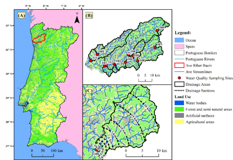
The present study aims to demonstrate how the distribution and shape of land use patches affect ecological integrity as well as the variation of these relationships with the adopted scale. The first step to fulfil this task was to measure the IPtIN (North Invertebrate Portuguese Index) in 12 points in Ave River Basin, Figure 1 (A), numbered from 101 to 112, Figure 1 (B), during the winter and summer of 2017. This index was chosen because the calculation is based on the quantity and diversity of benthic macroinvertebrates, which are sensitive to different types of pollution. For such reason, this index was used as an evaluator of water quality, for more information on measurement processes, please see the paper [31]. For each sampling site, it was delineated the upstream drainage area, using ArcMap [37] and ArcHYDRO [38] tools, Figure 1 (B). In order to trace the variations for each different scale, it was intersected each drainage area, with buffers surrounding each sampling site, delineating different drainage sections for each sampling site, varying from 100 meters to 56 km, in Figure 1 (C) the sections are shown for sampling site 108. For the calculation of landscape metrics, it was used the Portuguese Land Cover map of 2015 (COS 2015) as input for the Python toolbox [39]. It was calculated a total of 17 metrics (Table 1) for generic land uses: artificial surfaces, forested and semi-natural areas, and agricultural areas.
The effect of each landscape metric in water quality was accessed through the Spearman’s rank correlation coefficient [40]. It was chosen to use this coefficient since it is a nonparametric approach to determine the associated monotonic relationship two variables. Besides Pearson correlation is widely used to measure the linear correlation between two variables [41], it was not used the Pearson correlation since it requires certain assumptions such as normal distribution an absence of outliers [42], that can be found in the analysed variables. It was interpreted a total of 1508 correlations, between the landscape metrics calculated for different scales, with the IPtIN values collected in summer and winter.
Figure 1. Study area representation; (A) Portugal; (B) Ave River Basin; (C) Drainage area of sampling site 108 and traced drainage sections
Table 1. Calculated Landscape metrics [39]
|
Metric |
Defenition |
Description |
|
Class Area |
ca |
area of the patches of the corresponding class within the statistical zone |
|
Number of Patches |
npc |
number of patches for each corresponding classwithin the statistical zone |
|
Zone Area |
zone_area |
area of the statistical zone in which landscape metrics are calculated |
|
Percentage of Zone |
pz |
percentage of the area of the corresponding class per statistical zone |
|
Largest Patch index |
lpi |
percentage of statistical zone total area taken by the largest patch |
|
lpi_class |
name of the largest patch class |
|
|
Total Class Edge |
tc_edge |
length of edges of all patches in selected classes within the statistical zone |
|
Edge Density |
ed |
edge density |
|
Shannon Diversity |
shdi |
Shannon diversity index (SHDI) per zone. |
|
Edge Lenght |
el_a_class |
edge length of the focus class |
|
el |
edge length of focus class boundary shared with contrast class/es |
|
|
Contrast Class Edge |
cce |
percentage of edge length of the focus class shared with contrast classes. |
|
Connectance Index |
ci_np |
number of connected patches |
|
ci_pa |
patch area within range of connection |
|
|
ci_pp |
percentage of patch area within range of connection to statistical zone area |
|
|
ci_ca |
area of the connection zone between patches |
|
|
ci_cp |
percentage of connection zone between patches to statistical zone area |
The IPtIN measurements in summer and winter in Ave River basin are presented in Table 2. This index varies from 0 (indicating poor water quality) to 1.05 (indicating excellent water quality). Values ranged from 0.113 to 1.05 in winter and 0.275 to 1.017 in summer. The selected sampling sites were suitable for this study since it is caught the entire spectrum of IPtIN classifications, only the “good” status was not found in the sampling sites measurements (Table 2).
Table 2. IPtIN measurements in the twelve sampling sites and respective classification
|
Site |
Winter 2017 |
Summer 2017 |
||
|
101 |
0.42 |
Poor |
0.98 |
Excellent |
|
102 |
0.63 |
Moderate |
0.4 |
Poor |
|
103 |
0.39 |
Poor |
0.36 |
Poor |
|
104 |
0.11 |
Poor |
0.5 |
Moderate |
|
105 |
1.05 |
Excellent |
1.02 |
Excellent |
|
106 |
0.31 |
Poor |
0.51 |
Moderate |
|
107 |
1.05 |
Excellent |
0.94 |
Excellent |
|
108 |
0.49 |
Moderate |
0.58 |
Moderate |
|
109 |
0.14 |
Poor |
0.35 |
Poor |
|
110 |
0.52 |
Moderate |
0.31 |
Poor |
|
111 |
0.43 |
Moderate |
0.4 |
Poor |
|
112 |
0.22 |
Poor |
0.28 |
Poor |
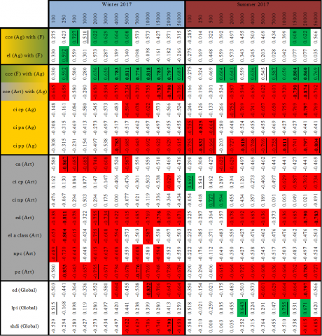
Spearman correlations were calculated for all the landscape variables in different distances paired with the IPtIN measurements. The critical values of Spearman’s Rank Correlation Coefficient (rs) for two-tailed probabilities of 0.05 and 0.005 are 0.587 and 0.776, respectively [43]. The first value was chosen as a threshold of significance since the probability of 0.05 is commonly accepted to reject the null hypothesis (h0: there is no effect between variables). In Figure 2 (A) and (B), are shown the scatter plots between the IPtIN in winter with the SHDI in a distance of 100 meters and 56 km, respectively, while in Figure 2 (C) and (D) are shown the same scatter for IPtIN measurements in summer. In Figure 2 (E) is shown the correlation variations between IPtIN and SHDI for distances 13 different scales. For the distances of 100, 250, 500, 1000, 2000, 3000, 4000, 5000, 7000, 10,000, 15,000, 20,000, and 56,000 meters, the log10 values are 2, 2.4, 2.7, 3, 3.3, 3.5, 3.6, 3.7, 3.8, 4, 4.2, 4.3 and 4.7, respectively.
Through the analysis of Figure 2 (E) is concluded that SHDI decreases IPtIN since rs values are negative (exception of rs calculated for IPtIN in summer with SHDI for distances between 500 m and 2 km). Besides the majority of correlations are negative these are only statistically significant for long distances, in summer period at 20 and 56 km, while in winter at distances higher than 4 km, particularly at 20 km where rs is equal to -0.790. This indicates that SHDI negative effect in water quality occurs for both seasons, but the effects are stronger during the winter period, only at the longest spatial extent (56 km) correlations converge. Besides correlations between SHDI and IPtIN demonstrate relevant results, among other metrics it was obtained significant correlations. In Figure 3 is shown the variables where it was found strongest correlations in each spatial extent, maximums and minimums are underlined. Significant correlations (α≤0.05) were highlighted in red and green, for positive and negative values, respectively. Correlations with high significance (α≤0.005) were marked in bold.
By paying particular attention to the correlations with statistical significance, is seen that majority of the correlations are concordant to theoretical expectations. Metrics respective to forestry land uses have positive correlations, while agricultural and artificial land uses correlations are negative. Only for “ci np (Art)” at 500 an 1000 meters and “ci np (Art)” at 100 meters are found positive correlations, which is hard to explain. As seen in Figure 3, metrics effects are influenced not only by the season but also by the spatial extent, as seasons changes occur predominantly hydrological changes [44]. Another time-dependent factor is the application of fertilizers, pesticides and herbicides [45], which is also dependent on specific cultures and plagues. During the winter period (for the demonstrated metrics) more correlations have statistical significance, a total of 94, while in summer 80. This might be due to the fact that during the winter the resulting runoff from precipitation is much higher than in summer [46], transporting sediments, nutrients and pesticides [47] from agricultural land uses, and contaminants from artificial land use to surface waters. With the presence of contaminants in surface waters, benthic macroinvertebrates communities are harmed, what is reflected in a decrease of quantity and biodiversity, and consequently, the index value (IPtIN) deceases. Is important to note that during summer periods the rivers are recharged dominantly by underground waters flow. For such reason, contaminants that are retained in aquifers are more vulnerable to be unleashed during summer periods. Another crucial aspect is that for particular agricultural cultures, fertilization/ pesticides/herbicides periods are in summer, and even soil erosion or summer rainfalls might be enough to transport them to surface waters. Metrics that only demonstrated a significant effect only during winter are “el (Ag) with (F)”, “el a class (Art)” and “npc (Art)”; metrics that only demonstrated a significant effect during summer are “ci pa (Ag)”, “ci np (Art)” and “lpi (Global)”, but other metrics have an effect in both seasons. Edge density “Ed” is the only metric that has an equal number of spatial extents with significance for summer and winter. The accessed scale reflects spatial effects, some metrics revealed that the effect in a short or long distance can be different. When the effects are strong only at long scales indicates that there is a propagation of contamination in long distances, with an inefficient auto-depuration. In cases that are only found a metric effect in short scale, it is probable that the resulting contamination effect is local and the contaminants are not transported in long distances, possibly can be locally retained, or are dispersed in transportation achieving harmless concentrations. In general, it is concluded that most of the relevant/stronger effects are found in the long scale. Only “ci pa (Ag)” revealed as the only metric that revealed a clear effect in short scale during the summer period. This metric consists on the area occupied by agriculture independently on the shape of agricultural land uses patches. The reason that this metric only has effect in short distance during summer might rely on agricultural substances that are applied in agricultural field have a strong effect in short distance.
Figure 2. Spearman rank correlation coefficient between Shanon’s Diversity index and IPtIN for different spatial extents; (A) Scatterplot for IPtIN in winter and SHDI at a 100 meters scale; (B) Scatterplot for IPtIN in winter and SHDI at a 56 km scale; (C) Scatterplot for IPtIN in summer and SHDI at a 100 meters scale; (D) Scatterplot for IPtIN in summer and SHDI at a 56 km scale; (E) Spearman’s correlation coefficient variation along scale and season, between SHDI and IPtIN
Figure 3. Spearman correlation ranks, between landscape metrics measured in various spatial extents and measured IPtIN during summer and winter
Among all metrics, the contrast metric “cce” of agricultural fields with artificial land use “cce (Art) with (Ag)” and forestry land uses “cce (F) with (Ag)” have an effect that is statistically significant in many spatial scales, predominantly in longer spatial extents. This metric is the percentage of agricultural land use patches edges that are shared with other land uses. This metric demonstrated that the combined effect of agricultural land uses with artificial surfaces leads to a significant loss of water quality, not only by the fact that both of this land uses are the greatest sources of contamination but also because in artificial surfaces the runoff velocity and flow are much higher because the infiltration is close to zero. For such reasons, the combination of agricultural areas with artificial surfaces is a great threat to water quality. On the other hand, it was found that the combination of agricultural fields with forested areas improves water quality. This result is quite peculiar and unpredicted since maximum correlations were achieved in this metric, with high statistical significance for winter and summer since these values are higher than 0.776 (α≤ 0.5%). It was expected that the highest correlations would be found in metrics that were calculated only for forestry land uses [48], but the dataset revealed the opposite. First, is reminded that in this study, water quality was accessed through an ecological indicator, based on the quantity and diversity of benthic macroinvertebrates. This possibly happens because agricultural fields contain nutrients from fertilizers application, which end up transported to freshwaters through runoff and soil erosion. If agricultural fields are attached to forested areas, these result as moderators of nutrients transport [21], part of them is retained in forested fields, as a consequence the nutrients from agricultural fields that pass through forested areas are induced in freshwaters, resulting in optimal concentrations for the development of macroinvertebrates.
These results are quite similar to a particular study where the effect of agriculture combined with forested land uses effects explain water quality variations, enhanced than when these variables are used alone [49]. Such results prove that sustainable agriculture can not harm, but even, improve water quality when combined with forested land uses, as barriers of contamination from runoff or soil erosion. In studies of similar scope, it was used PLS-PM (Partial Leas Squares Path - Modelling) to establish cause-effect interactions between pressures with ecological status[50-52], in Ave River Basin. The authors concluded that livestock and effluent discharges were major threats to water quality, but in such analysis, the only studied landscape metric was only the area percentage for different land-use types “pz”. When more detailed landscape metrics were paired with point source emissions, it was concluded that the effect of landscape metrics can be stronger than effluent discharges [31].
Such approaches that resort to multivariate statistical methods are quite useful to interpret which variables have a stronger effect. However, the disadvantage is that such statistical methods are vulnerable to collinearity and for this reason, the number of variables used in the models has to be reduced due to the variance inflation factor [53], and even significant variables must be discarded from such models [51].
In a previous study, the application of different statistical models was tested to evaluate which could be the most suitable form for prediction purposes [54], concluding that point source emissions and livestock production were the threats to water quality. In that study [54], landscape metrics were not included in the statistical models, and since such variables were not explored, it surged the necessity to study them. Resorting to a simpler method, by using Spearman Rank’s Coefficient, it was possible to trace the effect of many variables. Still, in different approaches is possible to trace different conclusions, even with a similar dataset. In a study where the effect of SHDI was studied [31], the impact of SHDI was higher on a short scale rather than in a long scale, through PLS-PM. But when this effect is analysed in simple statistics, it is seen that the impact is also negative but increases from the short scale to the longest.
This type of studies is quite useful to understand the role of pressures in surface waters, in this case, landscape metrics. It is quite important to tackle this issue since this study proved that the interactions with water quality are statistically significant. The utility of such approaches also to provides information about which can be the better locations for water caption [55], or in terms of land use planning, how should be implemented. Although it was assumed that the long scale effects are dominant, this study design also proved that is extremely important to explore different spatial extents since in a single spatial the strongest impact might now be accessed.
The measurements of the IPtIN index during the winter and summer of 2017 revealed that Ave River Basin water quality is vulnerable to seasonal changes since in 5 of the 12 measurement sites the ecological status changed. The present study design proved to be effective to demonstrate the spatial and seasonal effects of landscape metrics in water quality, by pairing landscape metrics with IPtIN for different spatial extents. Besides the most tackled threat in Ave River basin is effluent discharges, the present study shown that landscape is also a crucial aspect for this river basin’s water quality. Although in this approach, the authors resorted to the calculation of Spearman’s Rank Correlation Coefficient as a measure of effect, it was possible to analyse the effect of many variables on water quality. The results showed that the major threat but also a major benefit for water quality is agriculture, depending on the combined land use, urban or forestry. The correlations that led to this conclusion were the contrast of agricultural areas with artificial surfaces, where the Spearman correlation rank for long distances was higher than -0.7. While positive effects were found in the contrast between agricultural fields with forested areas, since the correlations with IPtIN, were close to 0.8, in a long-scale. The results provided relevant information since the strategic placement and configuration of agricultural fields is key to improve Ave River Basin water quality, which is the proposed challenge to municipal and regional water planners that are responsible for the safeguard and management of hydric resources.
This research was funded by the INTERACT project – “Integrated Research Environment, Agro-Chain and Technology”, no. NORTE-01-0145-FEDER-000017, in its line of research entitled BEST, co-financed by the European Regional Development Fund (ERDF) through NORTE 2020 (North Regional Operational Program 2014/2020). For the authors integrated with the CITAB Research Centre, it was further financed by the FEDER/COMPETE/POCI—Operational Competitiveness and Internationalization Programme, under Project POCI-01-0145-FEDER-006958, and by the National Funds of FCT—Portuguese Foundation for Science and Technology, under the project UID/AGR/04033/2020. For the author integrated in the CQVR, the National Funds of FCT—Portuguese Foundation for Science and Technology, under the project UID/QUI/00616/2019, supported the research. Financial support was also provided by the FCT-Portuguese Foundation for Science and Technology (Grant: SFRH/BD/146151/2019) to António Fernandes.
[1] Richardson, S.D., Ternes, T.A. (2018). Water analysis: emerging contaminants and current issues. Analytical Chemistry, 90(1): 398-428. https://doi.org/10.1021/acs.analchem.7b04577
[2] Schwarzenbach, R.P., Egli, T., Hofstetter, T.B., von Gunten, U., Wehrli, B. (2010). Global water pollution and human health, Annu. Rev. Environ. Resour., 35: 109-136. https://doi.org/10.1146/annurev-environ-100809-125342
[3] Trösch, W. (2009). Water treatment. Technology Guide: Principles - Applications - Trends, Springer Science and Business Media LLC, 394-397. https://doi.org/10.1007/978-3-540-88546-7_73
[4] Pacheco, F.A.L., Martins, L.M.O., Quininha, M., Oliveira, A.S., Sanches Fernandes, L.F. (2018). An approach to validate groundwater contamination risk in rural mountainous catchments: the role of lateral groundwater flows. MethodsX, 5: 1447-1455. https://doi.org/10.1016/j.mex.2018.11.002
[5] Nas, S.S., Nas, E. (2009). Water quality modeling and dissolved oxygen balance in streams: A point source streeter-phelps application in the case of the harsit stream. CLEAN - Soil, Air, Water, 37(1): 67-74. https://doi.org/10.1002/clen.200800107
[6] Vannote, R.L., Minshall, G.W., Cummins, K.W., Sedell, J.R., Cushing, C.E. (1980). The river continuum concept. Canadian Journal of Fisheries and Aquatic Sciences, 37(1): 130–137. https://doi.org/10.1139/f80-017
[7] Sousa, J.C.G., Ribeiro, A.R., Barbosa, M.O., Ribeiro, C., Tiritan, M.E., Pereira, M.F.R., Silva, A.M.T. (2019). Monitoring of the 17 EU Watch List contaminants of emerging concern in the Ave and the Sousa Rivers. Science of The Total Environment, 649: 1083-1095. https://doi.org/10.1016/j.scitotenv.2018.08.309
[8] Fonseca, A., Botelho, C., Boaventura, R.A.R., Vilar, V.J.P. (2014). Global warming effects on faecal coliform bacterium watershed impairments in Portugal. River Research and Applications, 31(10): 1344-1353. https://doi.org/10.1002/rra.2821
[9] Gupta, S.K. (2010). Modern Hydrology and Sustainable Water Development. John Wiley & Sons, Ltd. https://doi.org/10.1002/9781444323962
[10] Muga, H.E., Mihelcic, J.R. (2008). Sustainability of wastewater treatment technologies. Journal of Environmental Management, 88(3): 437-447. https://doi.org/10.1016/j.jenvman.2007.03.008
[11] Hayet, C., Saida, B.A., Youssef, T., Hédi, S. (2016). Study of biodegradability for municipal and industrial Tunisian wastewater by respirometric technique and batch reactor test. Sustainable Environment Research, 26(2): 55-62. https://doi.org/10.1016/j.serj.2015.11.001
[12] Sheoran, A.S., Sheoran, V. (2006). Heavy metal removal mechanism of acid mine drainage in wetlands: A critical review. Minerals Engineering, 19(2): 105-116. https://doi.org/10.1016/j.mineng.2005.08.006
[13] Gonçalves, E.P.R., Boaventura, R.A.R., Mouvet, C. (1992). Sediments and aquatic mosses as pollution indicators for heavy metals in the Ave river basin (Portugal). Science of The Total Environment, 114: 7-24. https://doi.org/10.1016/0048-9697(92)90410-t
[14] Grizzetti, B., Bouraoui, F., De Marsily, G. (2008). Assessing nitrogen pressures on European surface water. Global Biogeochemical Cycles, 22(4). https://doi.org/10.1029/2007gb003085
[15] Serrano-Grijalva, L., Sánchez-Carrillo, S., Angeler, D.G., Sánchez-Andrés, R., Álvarez-Cobelas, M. (2011). Effects of shrimp-farm effluents on the food web structure in subtropical coastal lagoons. Journal of Experimental Marine Biology and Ecology, 402(1-2): 65–74. https://doi.org/10.1016/j.jembe.2011.03.019
[16] Robb, G.A., Novotny, V., Olem, H. (1996). Water quality: Prevention, identification and management of diffuse pollution. The Geographical Journal, 162(1): 109. https://doi.org/10.2307/3060267
[17] Ferrier, R.C., Arcy, B.J., MacDonald, J., Aitken, M. (2005). Diffuse pollution - What is the nature of the problem? Water and Environment Journal, 19(4): 361-366. https://doi.org/10.1111/j.1747-6593.2005.tb00574.x
[18] Moss, B. (2007). Water pollution by agriculture. Philosophical Transactions of the Royal Society B: Biological Sciences, 363(1491): 659-666. https://doi.org/10.1098/rstb.2007.2176
[19] Nilsson, C., Svedmark, M. (2002). Basic principles and ecological consequences of changing water regimes: Riparian plant communities. Environmental Management, 30(4): 468-480. https://doi.org/10.1007/s00267-002-2735-2
[20] McGrane, S.J. (2016). Impacts of urbanisation on hydrological and water quality dynamics, and urban water management: A review. Hydrological Sciences Journal, 61(13): 2295-2311. https://doi.org/10.1080/02626667.2015.1128084
[21] Neary, D.G., Ice, G.G., Jackson, C.R. (2009). Linkages between forest soils and water quality and quantity. Forest Ecology and Management, 258(10): 2269-2281. https://doi.org/10.1016/j.foreco.2009.05.027
[22] Warrington, B., Aust, W., Barrett, S., Ford, W., Dolloff, C., Schilling, E., Wigley, T., Bolding, M. (2017). Forestry best management practices relationships with aquatic and riparian fauna: A review. Forests, 8(9): 331. https://doi.org/10.3390/f8090331
[23] Duarte, G.T., Santos, P.M., Cornelissen, T.G., Ribeiro, M.C., Paglia, A.P. (2018). The effects of landscape patterns on ecosystem services: meta-analyses of landscape services. Landscape Ecology, 33(8): 1247-1257. https://doi.org/10.1007/s10980-018-0673-5
[24] Johnson, L., Richards, C., Host, G., Arthur, J. (1997). Landscape influences on water chemistry in Midwestern stream ecosystems. Freshwater Biology, 37(1): 193-208. https://doi.org/10.1046/j.1365-2427.1997.d01-539.x
[25] Uuemaa, E., Roosaare, J., Mander, Ü. (2005). Scale dependence of landscape metrics and their indicatory value for nutrient and organic matter losses from catchments. Ecological Indicators, 5(4): 350-369. https://doi.org/10.1016/j.ecolind.2005.03.009
[26] Schiff, R., Benoit, G. (2007). Effects of impervious cover at multiple spatial scales on coastal watershed streams. Journal of the American Water Resources Association, 43(3): 712-730. https://doi.org/10.1111/j.1752-1688.2007.00057.x
[27] Yu, S., Xu, Z., Wu, W., Zuo, D. (2016). Effect of land use types on stream water quality under seasonal variation and topographic characteristics in the Wei River basin, China. Ecological Indicators, 60: 202-212. https://doi.org/10.1016/j.ecolind.2015.06.029
[28] Ding, J., Jiang, Y., Liu, Q., Hou, Z., Liao, J., Fu, L., Peng, Q. (2016). Influences of the land use pattern on water quality in low-order streams of the Dongjiang River basin, China: A multi-scale analysis. Science of The Total Environment, 551-552: 205-216. https://doi.org/10.1016/j.scitotenv.2016.01.162
[29] Allan, D., Erickson, D., Fay, J. (1997). The influence of catchment land use on stream integrity across multiple spatial scales. Freshwater Biology, 37(1): 149-161. https://doi.org/10.1046/j.1365-2427.1997.d01-546.x
[30] Fernandes, A.C.P., Sanches Fernandes, L F., Terêncio, D.P.S., Cortes, R.M.V., Pacheco, F.A.L. (2019). Seasonal and scale effects of anthropogenic pressures on water quality and ecological integrity: A study in the sabor river basin (NE Portugal) using partial least squares-path modeling. Water, 11(9): 1941. https://doi.org/10.3390/w11091941
[31] Fernandes, A.C.P., Sanches Fernandes, L.F., Cortes, R.M.V., Leal Pacheco, F.A. (2019). The role of landscape configuration, season, and distance from contaminant sources on the degradation of stream water quality in urban catchments. Water, 11(10): 2025. https://doi.org/10.3390/w11102025
[32] Soares, H.M.V., Boaventura, R.A., Machado, A.A.S., Esteves da Silva, J.C. (1999). Sediments as monitors of heavy metal contamination in the Ave river basin (Portugal): multivariate analysis of data. Environmental Pollution, 105(3): 311-323. https://doi.org/10.1016/s0269-7491(99)00048-2
[33] Alves, C.M., Boaventura, R.R.A.R., Soares, H.M.V.M. (2009). Evaluation of heavy metals pollution loadings in the sediments of the Ave River Basin (Portugal). Soil and Sediment Contamination: An International Journal, 18(5): 603-618. https://doi.org/10.1080/15320380903113568
[34] Fonseca, A., Boaventura, R.A.R., Vilar, V.J.P. (2017). Integrating water quality responses to best management practices in Portugal. Environmental Science and Pollution Research, 25(2): 1587-1596. https://doi.org/10.1007/s11356-017-0610-1
[35] Dunck, B., Lima-Fernandes, E., Cássio, F., Cunha, A., Rodrigues, L., Pascoal, C. (2015). Responses of primary production, leaf litter decomposition and associated communities to stream eutrophication. Environmental Pollution, 202: 32-40. https://doi.org/10.1016/j.envpol.2015.03.014
[36] Ramos, S., Amorim, E., Elliott, M., Cabral, H., Bordalo, A.A. (2012). Early life stages of fishes as indicators of estuarine ecosystem health. Ecological Indicators, 19: 172-183. https://doi.org/10.1016/j.ecolind.2011.08.024
[37] ESRI, ArcMap (Version 10). (2010). New York St. Redlands, USA.
[38] Zhang, J., Li, Q., Gong, H., Li, X., Song, L., Huang, J. (2010). Hydrologic Information Extraction Based on Arc Hydro Tool and DEM. 2010 International Conference on Challenges in Environmental Science and Computer Engineering, Wuhan, China. https://doi.org/10.1109/cesce.2010.169
[39] Adamczyk, J., Tiede, D. (2017). ZonalMetrics - a Python toolbox for zonal landscape structure analysis. Computers & Geosciences, 99: 91-99. https://doi.org/10.1016/j.cageo.2016.11.005
[40] Zar, J.H. (2005). Spearman Rank Correlation. In Encyclopedia of Biostatistics. John Wiley & Sons, Ltd. https://doi.org/10.1002/0470011815.b2a15150
[41] Pearson Correlation. (2018). In A Practical Approach to Using Statistics in Health Research. John Wiley & Sons, Inc. 165-172. https://doi.org/10.1002/9781119383628.ch17
[42] Nefzger, M.D., Drasgow, J. (1957). The needless assumption of normality in Pearson’s r. American Psychologist, 12(10): 623-625. https://doi.org/10.1037/h0048216
[43] Zar, J.H. (1972). Significance testing of the spearman rank correlation coefficient. Journal of the American Statistical Association, 67(339): 578-580. https://doi.org/10.1080/01621459.1972.10481251
[44] Ospina Noreña, J.E., Domínguez-Ramírez, C.A., Vega-Rodríguez, E.E., Darghan-Contreras, A.E., Rodríguez-Molano, L.E. (2017). Analysis of the water balance under regional scenarios of climate change for arid zones of Colombia. Atmósfera, 30(1): 63-76. https://doi.org/10.20937/atm.2017.30.01.06
[45] Wiedenfeld, R.P. (2000). Water stress during different sugarcane growth periods on yield and response to N fertilization. Agricultural Water Management, 43(2): 173-182. https://doi.org/10.1016/s0378-3774(99)00053-0
[46] Santos, M., Fonseca, A., Fragoso, M., Santos, J.A. (2018). Recent and future changes of precipitation extremes in mainland Portugal. Theoretical and Applied Climatology, 137(1-2): 1305-1319. https://doi.org/10.1007/s00704-018-2667-2
[47] Garcês, A., Pires, I., Rodrigues, P. (2019). Teratological effects of pesticides in vertebrates: a review. Journal of Environmental Science and Health, Part B, 55(1): 75-89. https://doi.org/10.1080/03601234.2019.1660562
[48] Chang, H. (2008). Spatial analysis of water quality trends in the Han River basin, South Korea. Water Research, 42(13): 3285-3304. https://doi.org/10.1016/j.watres.2008.04.006
[49] Pissarra, T.C.T., Valera, C.A., Costa, R.C.A., Siqueira, H.E., Martins Filho, M.V., Valle Júnior, R.F., Pacheco, F.A.L. (2019). A regression model of stream water quality based on interactions between landscape composition and riparian buffer width in small catchments. Water, 11(9): 1757. https://doi.org/10.3390/w11091757
[50] Sanches Fernandes, L.F., Fernandes, A.C.P., Ferreira, A.R.L., Cortes, R.M.V., Pacheco, F.A.L. (2018). A partial least squares – Path modeling analysis for the understanding of biodiversity loss in rural and urban watersheds in Portugal. Science of The Total Environment, 626: 1069-1085. https://doi.org/10.1016/j.scitotenv.2018.01.127
[51] Fernandes, A.C.P., Sanches Fernandes, L.F., Moura, J.P., Cortes, R.M.V., Pacheco, F.A.L. (2019). A structural equation model to predict macroinvertebrate-based ecological status in catchments influenced by anthropogenic pressures. Science of The Total Environment, 681: 242-257. https://doi.org/10.1016/j.scitotenv.2019.05.117
[52] Fernandes, A., Ferreira, A., Fernandes, L.S., Cortes, R., Pacheco, F. (2018). Path modelling analysis of pollution sources and environmental consequences in river basins. Water Pollution XIV. Presented at the Water Pollution 2018. https://doi.org/10.2495/wp180091
[53] Kock, N. (2015). Common method bias in PLS-SEM. International Journal of E-Collaboration, 11(4): 1-10. https://doi.org/10.4018/ijec.2015100101
[54] Fernandes, A., Ferreira, A., Fernandes, L.S., Cortes, R., Pacheco, F. (2019). PLS-PM For EcologicaL Integrity Mapping: Case Study Of The Ave River Basin, Portugal. Water and Society V. Water and Society 2019. https://doi.org/10.2495/ws190131
[55] Soares, S., Terêncio, D., Fernandes, L., Machado, J., Pacheco, F. (2019). The potential of small dams for conjunctive water management in rural municipalities. International Journal of Environmental Research and Public Health, 16(7): 1239. https://doi.org/10.3390/ijerph16071239