Aravind Pitchai Venkataraman* | Veeramani Veerapathran | Girirajkumar Marimuthu S.
© 2020 IIETA. This article is published by IIETA and is licensed under the CC BY 4.0 license (http://creativecommons.org/licenses/by/4.0/).
OPEN ACCESS
The optimization problem for multi-variable industrial high-efficiency control systems is to find the optimal parameters that could minimize the errors. In order to get such a stable control system, various control tuning methods were proposed by many researchers, but still, it is a challenge to get an effective controlled system. In this work, a method is proposed in order to attain a stable control system, called Error Recursion - Reduction Computational (ERRC) technique. Two processes, level, and flow are considered; their respective process models are identified and validated. The performance of the proposed technique has verified by implementing real-time transducers' interfaced experimental process. Results are compared with the conventional PID tuning technique and by optimization algorithms. The proposed experimental results show that better closed-loop performance can be achieved than other tuning techniques.
model identification, measurement, control, error minimization computational algorithm, ERRC, PSO
Proportional (P), Proportional plus Integral (I), Proportional plus Derivative (PD) and Proportional plus Integral plus Derivative (PID) are generic three-term controllers, widely used in feedback industrial control systems. PID controller can be implemented as a single or acombination of three controls. Proper tuning of these parameters is essential and important to get a stable control system. Over past half-centuries, several sets of PIDs formulas have been discussed. Among all methods, Ziegler Nichols is the basic tuning method, 1942 [1].
Prolong research on PIDs control, new tuning techniques are emerged out such as Cohen and Coon technique, 1953 [2] and Astrom and Hagguland technique, 1984 [3]. Many researchers appreciated these techniques due to maximum efficiency attained by minimum efforts. In recent 20 years, researchers are aiming to implement expert systems and process model parameters [4-6] to obtain PID controller parameters. The outcome is a model-based PID formula. The most well-known control method is the Internal Model Control Technique by Morari and Zafiriou [7-9]. Apart from these techniques, several research works are carried out on the human logical thinking ability and human nerve structure [10-12] based control. Nowadays, to meet the system demands, research communities deal with numerical optimization algorithms [13, 14]. Generally, optimization algorithms are classified as gradient and non-gradient algorithm [15-21]. Genetic algorithms (GA), grid searchers, stochastic, nonlinear simplex are families of non-gradient type algorithms [22]. Non-gradient algorithms are different from intelligent controllers [23-25] and Non-gradient algorithms are used to find optimum solutions, based on objective function evaluations. In the case of a gradient, it requires the presence of constant first subsidiaries of the target work and potentially higher subordinates. It requires the least number of configuration cycles to merge to an ideal contrasted with non-gradient based techniques [26-28].
Zheng et al. [29] designed an adaptive dynamic output-feedback control for a Chemical Continuous Stirred Tank Reactor System [30-32] under varying time delays with Nonlinear Uncertainties and highlighted the betterment of the adaptive control technique then others. Sowmya et al. proposed Genetic Algorithm Tuned Fuzzy Controller for a Nonlinear Process and this control algorithm different from numerical algorithms [33-35]. A Hybrid controller design was proposed [36] with State Feedback Controller Design for Two various Dynamic nonlinear systems.
For process analyze and purpose of design controllers, researchers are following common practices. They find a model of a physical system represented in terms of mathematical equations and to be used for further analysis. Such a process model is represented as the first or second-order process plus dead time.
To justify the efficiency of the proposed method, the real-time transducer is interfaced to give a closed-loop experiment model of linear tank level and flow process are considered: The dynamics of two different processes are analyzed, to get two process models.
Initially, the flow variable is individually controlled as single-loop control and results are analyzed. Secondly, the Level variable is controlled, process is considered as cascade control mode of multivariable process. The inner loop variable is flow and outer (main) loop variable is liquid level and their respective results are highlighted.
2.1 Model verification and parameter range settings
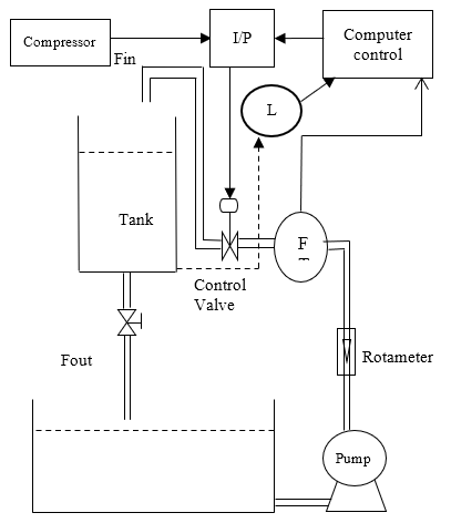
The real-time closed-loop experimental system consisting of various components are listed in Table 3 and (National Instruments- Educational Laboratory Virtual Instrumentation Suite) NI-ELVIS interface module, using LabVIEW which goes about as a controller, frames a closed-loop framework. The NI-ELVIS interfacing module and experimental process station with control valve and DPT appears in Figure 1 and Figure 2 respectively. The piping and instrument diagram of the framework appearing in Figure 3: in Table 1, process tank particulars are given. The inflow rate of the progressive tank is controlled by adjusting the stem spot of the pneumatic valve, passing a control signal the current to pneumatic converter through the NI-ELVIS analog channel. The working current range is 4-20 mA, is utilized to control the valve position. 4-20-mA is changed over to 3-15 psi by utilizing compacted pneumatic stress. The water level in the tank is measured by capacitance type electronic two-wire level sensor which is calibrated to 0-90 cm to give an output current range of 4-20 mA. Capacitance type differential pressure transmitter, the output range of (0-200) mm is used for flow measurement. The output current signal, from the level sensor and DPT, pass through the nominal value of the resistor and converted to a range of 1.28-5.36 V, level: for flow, the operating range 0.63-1.89 V, is given through the analog input channel of NI-ELVIS. The NI- ELVIS module is used to connect a personal computer and sensor/final control instruments. Signal (1-7)V, from the computer, is mapped to (3-15) psi pressure to operate the control valve.
NI-ELVIS has four analog channels and two analog channels to acquire and generate electrical signals respectively. NI-ELVIS module is designed to operate in the range of (-10 to +10) V accommodating both positive and negative terminals to acquiring and generating analog signals. The sampling rate of the module is on-demand of 1 sample/sec. It has a variable supply voltage of (0-12) V. It is used to acquire a signal from the level sensor and a flow sensor in the form of voltage and also used to operate I/P converter. It gives a pneumatic signal to the final control element (control valve).
Conversion formulation for mapping of acquiring and generating signals from and to the process is shown in Table 1 and Table 2.
Figure 1. Experimental process station
Figure 2. Interfacing unit
Table 1. Conversion formula for real time interfacing
|
Sl no |
Xai |
Xbi=Xai-Xai |
Xci=(Xbi)+((Xai)-(Xai+n))/(n)) |
Xdi=Xci/(Xci+1) |
|
1 |
Xai+1 |
Xbi+1=Xai+1-Xai+1 |
Xci+1=(Xbi+1)+((Xai+1)-(Xai+n))/(n)) |
Xdi+1=Xci+1/(Xci+1) |
|
2 |
Xai+2 |
Xbi+2=Xai+2-Xai+1 |
Xci+2=(Xbi+2)+((Xai+1)-(Xai+n))/(n)) |
Xdi+2=Xci+2/(Xci+1) |
|
3 |
Xai+3 |
Xbi+3=Xai+3-Xai+1 |
Xci+3=(Xbi+3)+((Xai+1)-(Xai+n))/(n)) |
Xdi+3=Xci+3/(Xci+1) |
|
4 |
Xai+4 |
Xbi+4=Xai+4-Xai+1 |
Xci+4=(Xbi+4)+((Xai+1)-(Xai+n))/(n)) |
Xdi+4=Xci+4/(Xci+1) |
|
5 |
Xai+5 |
Xbi+5=Xai+5-Xai+1 |
Xci+5=(Xbi+5)+((Xai+1)-(Xai+n))/(n)) |
Xdi+5=Xci+5/(Xci+1) |
|
| |
| |
| |
| |
| |
|
| |
| |
| |
| |
| |
|
6 |
Xai+n |
Xbi+n=Xai+n-Xai+1 |
Xci+n=(Xbi+n)+((Xai+1)-(Xai+n))/(n)) |
Xdi+n=Xci+n/(Xci+1) |
where, i=0, n=split count,
Equivalence of variables in formula and calculation section,
“Xai” is equal to “Xo”
“Xbi=Xai-Xai” is equal to “X1=Xo-initial value of Xo”
“Xci=(Xbi)+((Xai)-(Xai+n))/(n))” is equal to “X2=X1+0.51625”
Where, X2=4.13/8, i.e decide to split as 8 division and “Xdi=Xci/(Xci+1)” is equal to “X3=X2/intial value of X2”.
Table 2. Conversion formula for real time interfacing of level
|
Sl no |
Xo |
X1=Xo-initial value of Xo |
X2=X1+0.51625 |
X3=X2/initial value of X2 |
|
1 |
1.28 |
0 |
0.51625 |
1 |
|
2 |
1.7962 |
0.51625 |
1.0325 |
2 |
|
3 |
2.3125 |
1.0325 |
1.54875 |
3 |
|
4 |
2.8287 |
1.54875 |
2.065 |
4 |
|
5 |
3.345 |
2.065 |
2.58125 |
5 |
|
6 |
3.8612 |
2.58125 |
3.0975 |
6 |
|
7 |
4.3775 |
3.0975 |
3.61375 |
7 |
|
8 |
4.8937 |
3.61375 |
4.13 |
8 |
|
9 |
5.41 |
4.13 |
4.64625 |
9 |
Table 3. System specifications
|
Part Name |
Specifications |
|
Process Tank |
shape of Cylindrical and Transparent |
|
Level Transmitter (LT) |
Electronic- Level Range 0-90 cm, respective current signal of 4–20mA |
|
Differential Pressure Transmitter (DPT) |
Flow measurement, Range of (0-200) mm, respective current signal of 4–20mA |
|
Pump |
Centrifugal 0.5 HP |
|
Control valve |
Quarter Size, Normally open, Pneumatic, 3-15 psi |
|
Rotameter |
Range 10 - 100 LPH |
|
I/P converter |
Current range of 4-20 mA, Output pressure range of 3-15 psi |
|
Pressure gauge |
Operating Range 0 - 50 psi |
Figure 3. The piping and instrument diagram of the system
2.2 Modeling of process
In general, a process model is obtained by a step test method. A step change is applied to the process, and open-loop readings are taken. It gives a transient response. In this work, two identification methods being used to develop models and are validated. The model identified using SK (Sundaresan and Krishnaswamy) method [6] gives the best fitted to real-time readings. The level transmitter output of (4-20) mA is converted to a reasonable voltage by invoking a resistor and the value has been given to the data acquisition unit for indicating the real-time values. The same method is followed for the flow process, values are taken from DPT and the graph is plotted.
The formula used for SK method as follows,
$\mathrm{td}=1.3 \mathrm{t} 35.3-0.29 \mathrm{t} 85.3$ (1)
$\tau p=0.67(+85.3-t 35.3)$ (2)
The above-specified formula to be enforced separately, for level and flow process. Initially the flow rate of 30 LPH is adjusted and the readings for level and flow were taken. From the obtained set of readings, the transfer function parameters K (process gain), td (dead time) and τp (time constant) is to be found. General format to First Order Plus Time Delay (FOPTD) transfer function is,
$G(s)=\frac{\mathrm{K}_{\mathrm{p}} e^{-t_{d} s}}{\tau s+1}$ (3)
where,
$\mathrm{k}_{\mathrm{p}}=\frac{\text { change in output(level/flow) }}{\text { flow rate }}$
The response for the range of (0-90) cm of real time level system,
$G(s)=\frac{0.332 e^{-5.2 s}}{64.99 s+1}$ (4)
The reaction in the range of (0-200) mm of real time flow process,
$G(s)=\frac{0.126 e^{-14.27 s}}{60.97 s+1}$ (5)
Figure 4. Level process model validation
Figure 5. Flow process model validation
The response to the range of (0-90) cm of the real-time level process is shown in Figure 4 and the reaction in the range of (0-200) mm of real time flow process is shown in Figure 5.
This paper addresses the two tuning techniques [21] such as an internal model control (IMC) and PSO based PID tuning techniques [14] and respective PID [19] gain values are computed manually. In this section, tuning formulas, and implementation procedures are explained in the following subsections.
3.1 Conventional tuning
Keeping in mind the end goal to arrive a PID equivalent form for a process with a period delay, we should estimate the dead time by utilizing first order Pade approximation technique is shown in Eq. (7).
$G(s)=\frac{\mathrm{K}_{\mathrm{p}} e^{-t_{d} s}}{\tau s+1}$ (6)
$e^{-t_{d} s}=\frac{-0.5 \mathrm{t}_{\mathrm{d}} s+1}{0.5 \mathrm{t}_{\mathrm{d}} s+1}$ (7)
By solving the above two equations we can get PID controller parameters are follows,
$\mathrm{K}_{\mathrm{p}}=\frac{\tau+0.5 \mathrm{t}_{\mathrm{d}}}{\mathrm{K}_{\mathrm{p}}\left(\tau_{c}+0.5 \tau_{d}\right)}$ (8)
$\mathrm{T}_{\mathrm{i}}=\tau+0.5 \tau_{d}$ (9)
$\mathrm{T}_{\mathrm{d}}=\frac{\tau \tau_{d}}{2 \tau+\tau}$ (10)
3.2 Particle swarm optimization
PSO is a hearty stochastic enhancement procedure in view of the development and collaboration of swarms. PSO is a population-based swarm algorithm, developed by Eberhart et al. The use of PSO algorithm is put ahead by a few specialists who created computational recreations of the development of creatures, for example, schools of fish and rushes of flying creatures. Such reenactments are vigorously in view of controlling the divisions between individuals, i.e., the synchrony of the lead of the swarm was viewed as a push to keep an ideal separation between them.
3.3 Selection of PSO parameters
To fire up with PSO, certain constraints should be characterized. The choice of these settings chooses, as it were, the capacity of global minimization [21]. Design constants are of the Population size of 50, Number of iterations are 50 [27] and Velocity constants are c1=1.2 and c2=2.
velocity=w *velocity+c1*(R1.*(L_b_position-current_position))+c2*(R2.* (g_b_position-current_position)) (11)
where, c1 and c2 are sure constants address the scholarly and social parameter separately; R1 and R2 are discretionary numbers reliably passed on and w is idleness weight to adjust the worldwide and neighborhood seeks capacity.
3.4 ERRC
Error Recursion - Reduction Computational Technique (ERRC) is to improve the performance of the stabilized system or to stabilize an unstable system, a feedback controller is designed using the controller tuning technique. When the process undergoes changes in the operation or by the action of disturbances, the controller designed with classical tuning methods does not yield acceptable results. Hence, it is necessary to design the controller, which takes action to uncertainties and tackle disturbances.
This technique can be considered as a generalized framework for all types of processes. It can be easily incorporated into and adapt to any kind of controller.
The primary idea behind this technique is to minimize the error in order to get a perfect control action, in an integrated manner with the classical controller. Possible to estimate the error dynamically and can be minimized. This technique can be applied to both linear as well as non-linear systems.
3.4.1 Methodology
In the proposed technique, an error is optimally predicated or determined as a step-ahead output prediction method. Here, instant error e(kn) can be calculated from the present process output y(kn). Based upon the instant error value, the error value E(kn+1) has been predicted and to be processed to Parameter Identification (PI)space. In PI space, the ultimate output y(kn+N) should be found based upon the present data analysis. The predicted present ultimate output y(kn+N) to be forwarded to Parameter Evaluation (PE) space to check the fitness of the predicted value and should be sent to a loop analyzer to get the fitting error value to meet the system requirements. After all this process, error will be minimized and also the controller performance is improved. Figure 6 shows the block diagram of the ERRC technique for the multi-process station and Figure 7 shows the flow chart of the computational progress in the feedback. Where SP is setpoint, C is a comparator, C1, …, Cn-1, Cn are controllers for n processes and P1, …, Pn-1, Pn are representing processes. Xref is equal to the value of reference input and sensor.
The physical equation is consisting of present process output (Po), the respective error (eo), prediction of output (Pi) and error (ei) i=1,2,3,4….
$\text { Output, } \mathrm{P}_{\mathrm{i}+1}=\left[\left(\mathrm{P}_{\mathrm{i}-1}-\mathrm{t}_{\mathrm{p}}\right)+\mathrm{e}_{\mathrm{i}}\right] $ (12)
Figure 6. Block diagram of ERRC technique for multi process variables
Figure 7. Flow chart of computational progress
The objective of the computational technique is to trim down the error to zero. In general, an error is calculated on the basis of relationship exists between the actual output (yp) and target output (tp),
Error, $\mathrm{E}=\left(\mathrm{t}_{\mathrm{p}}-\mathrm{y}_{\mathrm{N}}\right)$ (13)
The parameter estimation equation is formed on the basis of process,
$\mathrm{E}_{0}=\left(\mathrm{t}_{\mathrm{p}}-\mathrm{P}_{0}\right)$ (14)
Which gives present error value e0.
Based upon this analog consecutive output, error values are predicted (i.e. Pi and ei are predicted, i.e. “i” varies from one to infinity). The steps to follow in the analysis, determine the best fit of the minimum error value and the output. This technique seems to be an iterative method, iteration continuous on error prediction, till the error converges to e<0.0……1.
yc is the present process output (C(t)), in both cases yc is added is to the error and depends on error signal polarity, whether the present process output value is added or subtracted to the error value.
The following section deals with the analysis of PID control settings that are found using IMC and PSO for both level and flow processes are tabulated in Table 4.
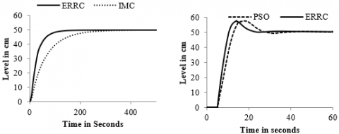
After computation of controller parameters, the validate models of both level and flow processes are taken for controller implementation. Closed-loop control performances of IMC based PIDs and PSO based PIDs controllers, implementation and analyses are done on LabVIEW platform. The controller parameters are computed and actualized for flow and level variable. Response shown in Figure 8 to Figure 9, after the inclusion of ERRC to the designed controller, which affects the process, and shows that the process quickly reaches the setpoint value.
The corresponding variation of flow rate and liquid level responses are taken for a set value of 25 LPH flow and 50 cm for flow and liquid level respectively.
On the basis of time-domain specifications and error response analysis. IMC based PID+ERRC implementation response yield a superior result than IMC based PID control action. Results are figured out in Table 5 and Figure 8 to Figure 12. Results prove that the addition of ERRC with the designed controller, which disturbs the process variable and helps it to steady-state at setpoint value with minimum rise time, minimum settling time and acceptable over an extensive variety of process activities.
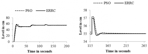
Servo and regulatory response for flow process and level process respectively, are appearing in Figure 10 and Figure 11 individually. Figure 10 and 11, clearly states that how fast the proposed method, reacts to disturbance and eliminate it, compared to other methods. For servo response, the set value is given as 5 lph change and 5 cm for flow and to the level process respectively. In regulatory response, a disturbance at time 400 seconds for the flow process and at 120 seconds for the level process. The proposed controller ERRC reacts faster and attains a steady state. The response of change in error for a flow and level process is shown in Figure 11 and the outcome is positive.
Table 4. PID controller parameter values for flow variable
|
Process |
Tuning methods |
Kp |
Ki |
Kd |
|
Flow |
Internal Model Control |
3.811 |
0.055 |
1.436 |
|
PSO based PID |
25.9189 |
0.538579 |
5.245511 |
|
|
Level |
Internal Model Control |
10.382 |
67.59 |
5.2524 |
|
PSO based PID |
27.81714 |
0.44931 |
19.54483 |
Table 5. Time domain specifications
|
Process |
Control mode |
Rise time (Tr) (Sec) |
Overshoot (%) |
Settling time (Ts) (Sec) |
|
Flow |
IMC based PID |
350 |
0 |
350 |
|
ERRC + IMC based PID |
75 |
25 |
170 |
|
|
PSO based PID |
32 |
34.08 |
110 |
|
|
ERRC + PSO based PID |
26 |
28.36 |
82 |
|
|
Level |
IMC based PID |
200 |
0 |
200 |
|
ERRC + IMC based PID |
90 |
0 |
90 |
|
|
PSO based PID |
13.07 |
15.6 |
38 |
|
|
ERRC + PSO based PID |
10.59 |
12.98 |
27 |
(a) (b)
Figure 8. Response of ERRC (a) with IMC and (b) with PSO for a flow process at Set value of 25 lph
(a) (b)
Figure 9. Response of ERRC (a) with IMC and (b) with PSO for a level process at Set value of 50 cm
(a) (b)
Figure 10. (a) Servo and (b) regulatory response for a flow process to a 5 lph and 0.3 % disturbance
(a) (b)
Figure 11. (a) Servo and (b) regulatory response for a level process to a 5 cm and 0.5 % disturbance
Figure 12. Response of change in error for (a) flow and (b) level process
The target of this work is effectively expert by executing the proposed procedure all the while. The performances of various control schemes were analyzed. The results in Figure 8 to Figure 12 shows the comparative response of various combinations of PID controllers. It is clearly stated that the process gives acceptable results with the addition of ERRC with conventional controls. In this work, presented that the proposed method was experimented in the controlling of level in the linear tank and in controlling of inflow rate to the tank. An analysis has come up with a conclusion that the time domain specifications rise time (Tr), settling time (Ts) and error are reduced drastically for the proposed method than other tuning methods.
[1] Ziegler, J.G., Nichols, N.B. (1924). Optimum setting for Automatic Controllers, Transactions of the ASME, 64: 759-768.
[2] Cohen, G.H., Coon, G.A. (1953). Theoretical consideration of retarded control. Trans ASME, 75: 827-834.
[3] Astrom, K.J., Hagglund, T. (1984). Automatic tuning of simple regulators with specifications on phase and amplitude margins. Automatica, 20(5): 645-651. https://doi.org/10.1016/0005-1098(84)90014-1
[4] Zadeh, LA. (1965). Fuzzy sets. Information and Control, 8(3): 339-353. https://doi.org/10.1016/S0019-9958(65)90241-X
[5] Mamdani, E.H. (1974). Application of fuzzy algorithm for control of simple dynamic plant. Proceedings of the Institution of Electrical Engineers, 121(12): 1585-1588. https://doi.org/10.1049/piee.1974.0328
[6] Sundaresan, K.R., Krishnaswamy, R. (1978). Estimation of time delay, time constant parameters in Time, Frequency and Laplace Domains, Journal of Chemical Engineering, 56(2): 257-262. https://doi.org/10.1002/cjce.5450560215
[7] Morari, M., Zafiriou, E. (1989). Robust Process Control. Prentice‐Hall, Inc., Englewood Cliffs, NJ, 488 pp. https://doi.org/10.1002/aic.690371216
[8] Matsummura, S, Ogata, K., Fujii, S., Shioya, H. (1998). Adaptive control for the steam temperature of thermal power plants. Proceedings of the 1998 IEEE International Conference on Control Applications, Trieste, Italy, pp. 1105-1109. https://doi.org/10.1109/CCA.1998.721628
[9] Astrom, K.J., Hagglund, T. (1995). PID Controllers: Theory, Design, and Tuning. International Society of America, Second edition. ISBN: 978-1-55617-516-9.
[10] Fabri, S., Kadirkamanathan, V. (1996). Dynamic structure neural networks for stable adaptive control of nonlinear systems. IEEE Transactions on Neural Networks, 7(5): 1151-1167. https://doi.org/10.1109/72.536311
[11] Levin, A.U., Narendra, K.S. (1996). Control of nonlinear dynamical systems using Neural Networks- Part II: observability, identification and control. IEEE Transactions on Neural Networks, 7(1): 30-42. https://doi.org/10.1109/72.478390
[12] Tan, Y.H., Dang, X.J., van Cauwenberghe, A. (1999). Generalised nonlinear PID controller based on neural networks. 1999 Information, Decision and Control. Data and Information Fusion Symposium, Signal Processing and Communications Symposium and Decision and Control Symposium. Proceedings (Cat. No.99EX251), Adelaide, SA, Australia. https://doi.org/10.1109/IDC.1999.754210
[13] Herrero, J.M., Blasco, X., Martinez, M., Salcedo, J.V. (2002). Optimal PID tuning with genetic algorithms for nonlinear process models. IFAC Proceedings Volumes, 35(1): 31-36. https://doi.org/10.3182/20020721-6-ES-1901.00658
[14] Kennedy, J.F., Eberhart, R.C., Shi, Y. (2001). Swarm Intelligence. Morgan Kaufmann Publishers Inc., San Francisco, CA, United States.
[15] Dorigo, M., Di Caro G. (1999). The Ant Colony Optimization Metaheuristic. In: Corne D, Dorigo M, Glover F, editors. New Ideas in Optimization. McGraw-Hill, 11-32.
[16] Bartz-Beielstein, T., Parsopoulos, K., Vrahatis, M.N. (2002). Tuning PSO parameters through sensitivity analysis. Technical Report of the Collaborative Research Center 531 Computational Intelligence CI--124/02, University of Dortmund. https://doi.org/10.13140/2.1.1466.2080
[17] Zheng, Y., Zhang, L.Y., Qian, J.X., Ma, L.H. (2003). Robust PID controller design using PSO. Proceedings of the 2003 IEEE International Symposium on Intelligent Control, Houston, TX, USA. https://doi.org/10.1109/ISIC.2003.1254769
[18] Bartz-Beielstein, T., Parsopoulos, K.E., Vrahatis, M.N. (2004). Design and analysis of optimization algorithms using computational statistics. Appl. Num. Anal. Comp. Math., 1(2): 413-433. https://doi.org/10.1002/anac.200410007
[19] Zhao, J., Li, T.P., Qian, J.X. (2005). Application of particle swarm optimization algorithm on robust PID controller tuning. In: Wang L., Chen K., Ong Y.S. (eds) Advances in Natural Computation. ICNC 2005. Lecture Notes in Computer Science, vol 3612. Springer, Berlin, Heidelberg. https://doi.org/10.1007/11539902_118
[20] Xu, Z.C. (2006). Parameter tuning method of robust PID controller based on particle swarm optimization algorithm. Control and Instruments in Chemical Industry, 33(5): 22-25.
[21] Giriraj Kumar, S.M., Sivasankar, R., Radhakrishnan, T.K., Dharmalingam, V., Anantharaman, N. (2008). Particle swarm optimization technique based design of Pi controller for a real-time non-linear process. Instrumentation Science & Technology, 36(5): 525-542. https://doi.org/10.1080/10739140802234980
[22] Kumar, M.P., Vijayachitra, S. (2009). Process optimization using genetic algorithm. P 2009 International Conference on Control, Automation, Communication and Energy Conservation, Perundurai, Tamil Nadu, India, pp. 1-6.
[23] Jain, R., Sivakumaran, N., Radhakrishnan, T.K. (2011). Design of self tuning fuzzy controllers for nonlinear systems. Expert Systems with Applications, 38(4): 4466-4476. https://doi.org/10.1016/j.eswa.2010.09.118
[24] Ravi, V.R., Thyagarajan, T. (2011). Application of adaptive control technique to interacting non linear systems. Electronics Computer Technology (ICECT), 3rd International Conference, Kanyakumari, India, pp. 386-392. http://dx.doi.org/10.1109/ICECTECH.2011.5941724
[25] Sridharan, M. (2020). Predicting performance of double pipe parallel and counter flow heat exchanger using fuzzy logic. ASME - Journal of Thermal Science and Engineering Applications, 12(3): 1-11. https://doi.org/10.1115/1.4044696
[26] Aravind, P., Giriraj Kumar, S.M. (2013). Performance optimization of PI controller in non linear process using genetic algorithm. International Journal of Current Engineering and Technology, 3(5): 1968-1972.
[27] Aravind, P., Valluvan, M. (2014). PSO based optimization of PID controller for a Linear tank. International Journal of Current Engineering and Technology, 4(2): 486-490.
[28] Aravind, P., Giriraj Kumar, S.M. (2014). Application of optimization technique to tune pid controller for a level process. International Journal of Computer Applications, 91(6): 20-24. https://doi.org/10.5120/15965-5336
[29] Zheng, W., Wang, H.B., Wen, S.H., Wang, H.R., Zhang, Z.M. (2018). Adaptive dynamic output-feedback control for chemical continuous stirred tank reactor system with nonlinear uncertainties and multiple time-delays. International Journal of Control Automation System, 16: 1681-1691. http://dx.doi.org/10.1007/s12555-017-0363-0
[30] Song, B., Tan, S., Shi, H.B. (2016). Key principal components with recursive local outlier factor for multimode chemical process monitoring. Journal of Process Control, 47: 136-149. https://doi.org/10.1016/j.jprocont.2016.09.006
[31] Brásio, A.S.R., Romanenko, A., Fernandes, N.C.P., Santos, L.O. (2016). First principle modeling and predictive control of a continuous biodiesel plant. Journal of Process Control, 47: 11-21. https://doi.org/10.1016/j.jprocont.2016.09.003
[32] Dinesh Kumar, D., Meenakshipriya, B. (2016). Design of heuristic algorithm for non-linear system. Rev. Téc. Ing. Univ. Zulia, 39(6): 10-15. http://dx.doi.org/10.21311/001.39.6.02
[33] Murillo-Marrodan, A., Garcia, E., Cortes, F. (2018). A study of friction model performance in a skew rolling process numerical simulation. International Journal of Simulation Modelling, 17(4): 569-582. http://dx.doi.org/10.2507/IJSIMM17(4)441
[34] Sowmya, P., Balasubramanian, G., Rakeshkumar, S., Ramkumar, K. (2014). A genetic algorithm tuned fuzzy controller for a nonlinear process. Journal of Applied Sciences, 14: 1576-1581. https://doi.org/10.3923/jas.2014.1576.1581
[35] Sridharan, M., Jayaprakash, G. (2019). Verification and validation of solar photovoltaic thermal water collectors performance using fuzzy logic. Journal of Verification, Validation and Uncertainty Quantification, 4(4): 1-8. https://doi.org/10.1115/1.4045895
[36] Aravind, P., Veeramani, V., Girirajkumar, S.M. (2019). A hybrid state feedback controller design for two different dynamic systems. International Journal of Operational Research. http://doi.org/10.1504/IJOR.2021.10023686