Ogunlade Michael Adegoke* | Ilesanmi Banjo Oluwafemi | Olaitan Akinsanmi
© 2020 IIETA. This article is published by IIETA and is licensed under the CC BY 4.0 license (http://creativecommons.org/licenses/by/4.0/).
OPEN ACCESS
The power line communication (PLC) channel is mainly affected by noise that is either caused by appliances or induced into channel from external source. The effects of those noises on transmission network constitute major problem that must be tackled. In this paper, a time domain noise measurement and characterization is presented. A design measurement system was set up that captured the noise in time domain for real indoor power line communication. Noise samples were captured with four channel digital storage oscilloscope (DSO) GDS-1052-U with two inputs channels. The time domain noise measurement is presented together with its statistical analysis based on numerous measurement campaigns in different laboratories at Afe Babalola University Ado Ekiti Nigeria, within three months; October, November and early December 2019. The measurement was taken between the hours of 8am-6pm, Monday –Saturday. Those days were equally distributed over three months of investigation. The measurement was carried out when all the electrical loads were running. The parameters of the noise measurements in terms of its duration, amplitude, impulsive and background noise voltage were examined. We compare our results to that of literatures; in comparison, the disparity with respect to durations and amplitude (mean and standard deviation) is quite significant.
background noise, electromagnetic interference, impulsive noise, power line network
The power line communication (PLC) can broadly be defined as a technology that makes use of electrical power network transmission for data communication by leveraging on already installed electrical power transmission. PLC allows vital information or data to be sent over distribution power lines. In order words, internet data is running on those power lines and at the same time carrying electrical power as well. This is achievable as a result of internet over power line (IPL) technology. The PLC can also be called broadband power line communication (BPL). PLC allows access to internet via wall socket at home and offices. The same socket that powers electronic gadget enables us to access the internet as well from the power line. A PLC channel system consists of channel transfer functions and noise [1]. For many years, PLC has become apparent alternative solutions for indoor power line communication systems [2, 3]. PLC technology has come into existence as a substitute to conservative wired and wireless communication systems due to its various advantages [2, 4]. Initially, the electrical power line transmission channel was not meant for data communication purposes. The medium is not suitable for dependable communication. There are some significant challenges of PLC channel which are: high noise level, high channel attenuation and signal reflection along the power line [2]. PLC channel displays very high attenuation as well as strong low pass characteristics which confines both the network coverage and the bandwidth to be used for communication systems. As a result of change in topology, cable parameters and load impedances, the PLC channel noise is time-dependent and therefore weakened by both impulsive noise and colored background noise [5]. The intrinsic noise in electrical power line network is harmful and this can comfortably wipe data streams out causing loss of communications. Noise in PLC system can be divided into two categories: impulsive noise and background noise. The impulsive noise seems to have the greatest impact on signal transmission. It is random in nature with large amplitude that interferes with PLC and hence, leads to an increase in bit error rate of signal transmission [6]. Noise in PLC is of different types depending on its source as well as its physical properties. The noise in communication system is refers to as additive white Gaussian noise. This type of noise is different from PLC noise, which is non-Gaussian, very complex and not predictable. However, the noise in PLC systems can also be regarded as white noise. This is true only in broadband range and hence, in narrowband range, the noise is colored noise. As a result of the difficulty associated with noise set-up in PLC systems, efforts to model the noise in both frequency and time domain have been on for some time. The tasks have made this technology a research area to be focus on in future. Therefore, for a reliable noise measurements and model extensive studies on noise characterizations are necessary. Due to the unique advantages of using the widely existing power line infrastructure, PLC has been considered to be a unique solution for smart grid communication and has raised a lot of interest over the years. The structure of electrical grid differs in each countries around the world. For example, two phase structural configurations are peculiar in United State of America, while three-phase configuration is used in European countries [5]. The average indoor power supply in Nigeria is 240V at 50Hz. The electrical power grid consists of high, medium and low voltage transmission respectively [5, 6]. The broadband PLC system is divided into two categories: Indoor PLC and last mile PLC. The focus of this research is on indoor noise measurements in residential, commercial, and offices buildings. On the other hand, last mile PLC noise measurement focus on out door high voltage [2, 5, 7].
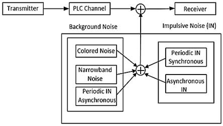
PLC noise can be divided into different classes, depending on its source as well as its physical properties [2, 8]. Figure 1 shows the categories of noise scenario in PLC. The power line noise can be classified into two major groups which are; background noise and impulsive noise [2].
2.1 Background noise
The major causes of background noise emanate from common domestic appliances such as light dimmers, desktop and laptop computers, etc. It is also caused by the summation of different noise sources of infinitesimal power. The power present in the signal of a background noise which is a function of frequency per unit frequency otherwise known as power spectral density (PSD) [9]. It is very low and hence, to a large extent increases towards lower range of frequencies [2, 7, 9]. The average range is between -140 and -125dBm/Hz [2, 10]. On the other hand, narrow-band noise is produced from electrical devices connected to the network terminals, and also from industrial equipments in relative vicinity. The periodic impulsive noise is produced by switching power supplies and is usually impulsive and periodically asynchronous to the mains frequency [2]. The range of the spectrum repetition rate is between 50 to 200kHz [11].
Figure 1. Noise scenario
2.2 Impulsive noise
The impulsive noise is caused by switching of rectifier diode. It has a varying time from microseconds to milliseconds, random in nature and has high power spectral densities [12]. The rise in PSD of impulsive noise causes bit errors in data transmission [2, 7]. In addition, it has a repetition rate of 50 or 100Hz and is of short duration, about 10 - 100$\boldsymbol{\mu} \mathrm{s}$. Research has shown that noise is very hard to be characterized using pure analytical derivation method. Hence, all of the existing noise models are obtained based on empirical measurements. The impulsive noise is characterized by three random variables which are: Interarrival time, amplitude and width [13]. However, the background noise and the impulsive noise have peculiar characteristics. The background noise is time variant in nature and the latter cannot be considered stationary simply because it has high PSD [2, 14]. The overall system noise as given in Eq. (1), can be modeled as the sum of the background noise, and the impulsive noise denoted as $n_{b}(t)$, and the impulsive noise, denoted as $n_{i m p}(t)$[2].
$n\lfloor(t)\rfloor=n_{b}(t)+n_{i m p}(t)$ (1)
An intensive time domain noise measurement was carried out in the Department of Electronic and Computer Engineering. Afe Babalola University (ABUAD), Ado Ekiti, Nigeria. The measurement for this study were retrospectively taken from different locations in ABUAD. The different locations where noise measurements were carried out are; Telecommunication laboratory, Digital electronic laboratory, Networking laboratory and National Instrument laboratory respectively. The noise measurements were carried out in time domain using four channel digital storage oscilloscope (DSO) GDS-1051-U. The DSO is a 50MHz digital storage oscilloscope by GW instek. It has two input channels, USB host and device port support that can be connected to computer. Table 1 shows the parameters of the DSO.
Table 1. GDS-1052 series digital oscilloscope parameters
|
Vertical Specifications |
Channels |
2 |
|
Bandwidth |
DC-50MHz (-3dB) |
|
|
Rise Time |
< 7nS |
|
|
Sensitivity |
2Mv/div – 10V/div |
|
|
Input coupling |
AC, DC, & Ground |
|
|
Polarity |
Normal & Invert |
|
|
Offset range |
2Mv/div- 50mV/div:+- 0.4V |
|
|
Bandwidth limit |
20MHz (-3db) |
|
|
Source |
CH1, CH2, Line, EXT. |
|
|
Coupling |
AC, DC, Noise rej, HF rej, |
|
|
Accuracy |
+_ 0.01% |
|
|
Pre-Trigger |
10div maximum |
|
|
Trigger |
Post-Trigger |
1000div |
|
X-Axis input |
Channel 1 |
|
|
Y- Axis input |
Channel 2 |
|
|
Phase shift |
+_3 at 100KHz |
|
|
Horizontal |
Real-Time sample rate |
250MSa/s maximum |
|
Vertical resolution |
8 Bits |
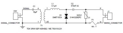
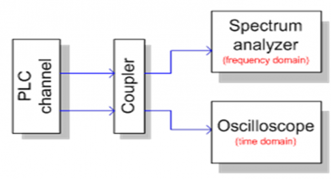
A power line communication AC coupling circult (Steval-XPLMO1CPL) was used mainly to detach the measurement equipments from the AC mains. The coupling circult is used as an interface between the PLC channel and the measurement device. The broadband coupling circuit does not only facilitate clear reception of the noise signals, but, enables galvanic isolation between mains and measurement equipment. The coupling circult schematic and block diagrams are shown in Figures 2 and 3. The coupling circuit is a simple yet very useful tool for power line communication testing on AC power networks. It includes simple two-wire connectivity to any PLC transmitter or receiver and a standard connector for an AC power cord.
Figure 2. Coupling circuit
Figure 3. Noise measurement block diagram
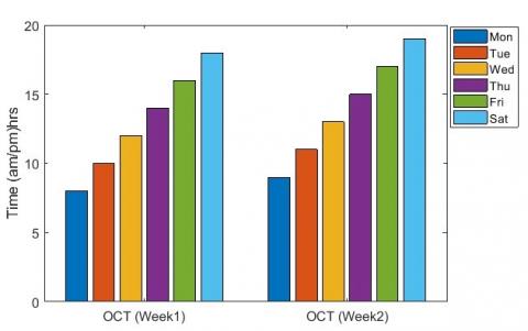
Figure 4. Week 1and 2 noise measurement durations
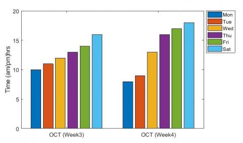
Figure 5. Week 3 and 4 noise measurement durations
The main components to achieve suitable signal coupling are: PLC 1:1 transformer for differential coupling and basic electrical isolation. It has a varistor for effective protection against surge disturbances from the power line. Also has a high voltage AC blocking capacitor with $\mathrm{X}_{2}$ safety class. The tuning series inductor is utilized to adjust the frequency response. The frequency response of the coupling circuit is wide enough to fit any narrow –band PLC signal under normal test conditions.
However, it can be easily adjusted by changing only the turning series inductor $\mathrm{L}_{1}$. The coupler is suitable for laboratory measurements using equipment like an isolated probe for an oscilloscope or a spectrum analyser or to inject a signal from an arbitrary function generator. The noise measurements were carried out between the hours of 8:00am and 6:00pm, Monday to Saturday for a period of three months as shown in Figures 4 and 5. Noise measurements were taken both on No-Load condition and when electronic devices were connected to the power line network.
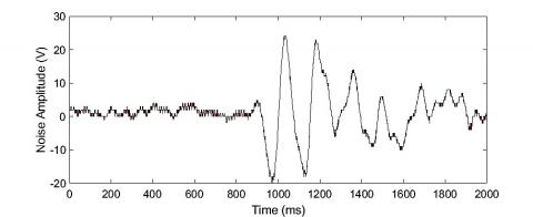
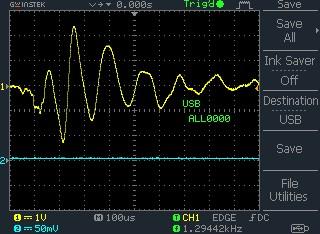
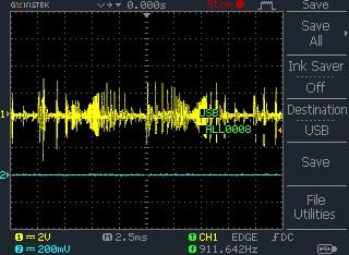
The results of the time domain noise measurements show that noise has periodic features as well as randomness for a few seconds to minutes. This remained periodic, stationary, and cyclic for long periods of observation. The noise waveform obtained in the laboratories that have a several desktop computers, Television set, soldering iron, laptop computer with charger, and fluorescent lamps etc., are shown in Figures 7-11. The noise waveform exhibits different characteristics. Out of numerous measurements taken, only a few measurements are shown due to space constraint. The practical measurements in power lines found that the typical strength of a single impulsive is more than 10 dB above the background noise level and can occasionally exceed 40dB [15, 16]. Similar behavior can be observed from our measurements where impulsive strength rises well above the background noise as shown in Figure 6(b). The impulsive amplitudes reached value that is well above the background noise level, as high as 0.75. For meaningful interpretation of the impulsive energy, a threshold value needs to be defined that represent background noise [13].
In Figure 6, we determined the background noise level to be 0.03V. Using this value as reference, the amount of increase in the noise level beyond this value is as follows [13].
$L_{v}=20 \log \left[\frac{V_{i}}{V_{b}}\right]$ (2)
where, $L_{v}$ represent the voltage level in decibel; $V_{i}$ represent the impulsive noise voltage, and $V_{b}$ represent the background noise voltage. Therefore, $L_{v}$ is equal to 27.95 dB.
Hence, the results are shown in Table 2. The analysis of the mathematical function of measured signals with respect to time is known as time domain [17]. The signal is actually a narrative of how a factor is related to another. The two factors that form a signal are generally not exchangeable (Noise amplitude and Time). The noise amplitude-axis which is known as dependent variables is a function of time on time-axis known as independent variable.
However, the independent variable (Time) describes when and how the sample is taken, while the amplitude-axis is the actual measurements. Therefore, any signal that makes use of time as the independent variables is said to be in time domain. Under no load condition, the measurement was performed in an isolated PLC network where there were no users at all in the network. The typical size or number of nodes in the network was very small and no equipment’s was left ON. Hence, isolating the network or depriving other users of the network sometimes is always difficult to enforce. There is a noticeable portion of interference emanate from electronic devices connected to the electrical power line terminals in relative proximity by radiation and conduction. Figure 7 to 12 show measurements of electrical loads connected to the electrical power line outlets. The different noise waveforms are observed with their respective amplitudes. All the electrical loads induced noise of different amplitudes into the power network. Therefore, electrical equipment’s connected to the power networks are a source of noise most especially during switching ON and OFF and exhibit different characteristics.

(a)

(b)
Figure 6. a) Asynchronous impulsive noise; b) Synchronous impulsive noise
Table 2. Parameters of impulsive and background noise
|
|
Impulsive noise voltage (V) |
Background noise voltage (V) |
Voltage level (dB) |
|
Our measurements |
0.75 |
0.03 |
27.95 |
|
Mosalaosi et. al. [11] |
0.60 |
0.05 |
21.50 |
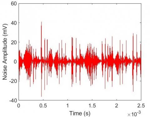
Figure 7. Phone charger noise waveform
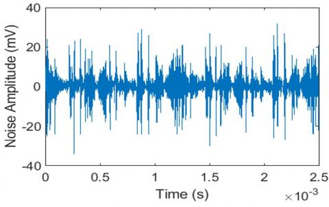
Figure 8. TV Set plus phone charger noise waveform
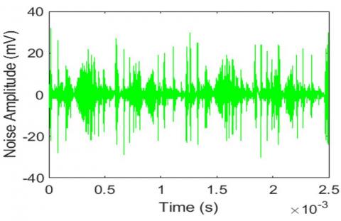
Figure 9. Laptop Computer noise waveform
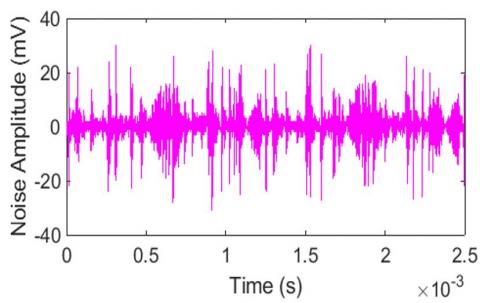
Figure 10. Fluorescent lamp noise waveform
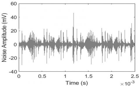
Figure 11. Laptop and TV loads waveform

Figure 12. Sum of all the noise in Figures 7-11
The noise induced into the power line network by the fluorescent lamp and phone charger are higher in amplitude than the other noises induced into the network. Hence, Figure 12 shows the summation of all the noises produced by different appliances. The noise at any power outlet of power network is the sum of all noises produced by different appliances connected to the power line plus background noises [13].
As Table 3 shows, there is a significant difference between the loads in terms of its Mean amplitude and the standard deviations. The measured values are the Mean, which is found by the addition of all the samples together and divide by the total number of samples (N). For the calculation of a signal’s Mean, the signal is contained in $X_{0}$ through $X_{N-1}$, where i is an index that runs through these values, and µ is the mean.
$\mu=\frac{1}{N} \sum_{i}^{N-1} X_{i}$ (3)
The standard deviation (SD) represents noise and other interference. SD is comparison to the mean. The SD is calculated as:
$\delta^{2}=\frac{1}{N-1} \sum_{I=0}^{N-1}[X i-\mu]^{2}$ (4)
The signal is stored in $\mathrm{X}_{\mathrm{i}}$, where $\mu$ is the mean, N is the number of samples, and $\delta$ is the standard deviation. The results of this study indicate that noise signals are spread out over a wider range of values. The amplitude of Mean values obtained from different electrical loads range from (33.0-798) mV. Therefore, the average amplitude Mean for all the loads is 441 mV. Likewise, amplitude standard deviation values range from (58.5-200.03) mV, with an average of 100mV respectively. This can have severe destructive impact on PLC signals and hence need for robust noise coding techniques and modulation schemes that can ease the effect of noise signal. The findings observed in this study mirror those of the previous studies that have measured noise in PLC. We compared our results to that of literature elsewhere as shown in Table 4. The result of the standard deviation of duration is quite large and different from the previous research results. This can be attributed to varied environment under study which has unpredictable noise source, structure, topology and unknown characteristics of the power cables. Hence, standard deviation of noise durations described the noise in terms of duration of occurrence which is of short duration and range from microseconds to a few miliseconds.
Table 3. Statistical parameters of impulsive noise amplitude
|
|
Loads |
Mean |
Standard deviation |
|
Amplitudes |
L1 |
0.033 |
61.95 |
|
L2 |
0.0628 |
61.08 |
|
|
L3 |
0.308 |
64.14 |
|
|
L4 |
0.241 |
62.73 |
|
|
L5 |
0.305 |
61.35 |
|
|
L6 |
0.302 |
63.04 |
|
|
L7 |
0.309 |
58.50 |
|
|
L8 |
0.753 |
200.03 |
|
|
L9 |
0.798 |
181.95 |
|
|
L10 |
0.798 |
181.95 |
Table 4. Impulsive noise parameters compared with literature elsewhere
|
|
Descriptions |
Mean |
Standard Deviation |
|
Amplitude (mV) |
Our measurements |
441 |
100 |
|
|
Mosalaosi et al. [10] |
391 |
198 |
|
|
Liu et al. [15] |
229 |
121 |
|
Durations ($\mu$s) |
Our measurements |
125 |
721 |
|
|
Mosalaosi et al. [10] |
152 |
139 |
|
|
Liu et al. [15] |
205 |
157 |
(a)
(b)
Figure 13. a) Sum of all the noise produced by different appliances connected to the line; b) Sum of all the noise using MATLAB
(a)
(b)
Figure 14. a) Indoor noise summation; b) Indoor noise summation using MATLAB
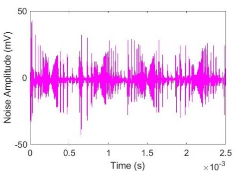
In addition, noise measurements were taken from digital electronics laboratory. The equipements connected to the power line are: Digital Multimeter MAS-TEK MS80550 (125 Watts), Oscilloscope GW instek GDS-1052U (18 Watts), ED-LAB CES505 electronic lab system (25 Watts), CISCO Router 2900 (240 Watts), and Functional generator (25 Watts) respectively. These appliances induced noise into the power line. The noise produced at the power outlet is the sum of all the noises produced by these appliances connected to the line plus background noise as shown in Figure 13 (a). Figure 13(b) shows the replica of the wave form using MATLAB.
The output waveform of indoor appliances that comprises of blender, microwave oven, electric cooker, electric kettle, standing fan and water dispenser are shown in Figure 14 with their amplitudes.
The waveforms show the summation of noise induced into the power line outlet by all the appliances.
Welch PSD method was used for the noise power spectral density estimation. This method provides a good estimate of the noise spectral and signal power at different frequencies [9]. Welch is computed as the magnitude squared of the Fourier Transform of a continuous time and finite power signal. For a Continuous stochastic process,
$X_{T}(t)=\left\{\begin{array}{c}x(t),|t| \leq \frac{T}{2} \\ 0,|t|>\frac{T}{2}\end{array}=X(t) \operatorname{rect}\left(\frac{t}{T}\right)\right.$ (5)
The Fourier Transform is
$F\left(X_{T}(t)\right)=\int_{-\infty}^{\infty} X_{T}(t) e^{-j 2 \pi f t} d t, \quad T<\infty$ (6)
Hence, using Parseval’s theorem,
$\left.\int_{\frac{-T}{2}}^{\frac{T}{2}}\left|X_{T}\right|(t)\right|^{2} d t=\int_{-\infty}^{\infty}\left|F\left(X_{T}(t)\right)\right|^{2} d f$ (7)
Dividing through by T,
$\frac{1}{T} \int_{-\frac{T}{2}}^{\frac{T}{2}} X_{T}^{2}(t) d t=\frac{1}{T} \int_{-\infty}^{\infty}\left|F\left(X_{T}(t)\right)\right|^{2} d f$ (8)
Hence, Eq. (8) is the average signal power over time, T.
The equation at the left side becomes the average power as T, approaches infinity. The FT at the right side equation is not defined in that limit. Therefore,
$E\left(\frac{1}{T} \int_{-\frac{T}{2}}^{\frac{T}{2}} X_{T}^{2}(t) d t\right)=E\left(\frac{1}{T} \int_{-\infty}^{\infty}\left|F\left(X_{T}\right)\right|^{2} d f\right)$ (9)
$\left.\lim _{T \rightarrow \infty} \frac{1}{T} \int_{-T / 2}^{T / 2} E\left(X^{2}\right) d t=\left.\lim _{T \rightarrow \infty} \frac{1}{T} \int_{-\infty}^{\infty} E\left[| F\left(X_{T}(t)\right)\right]\right|^{2}\right] d f$ (10)
$\left\langle E\left(X^{2}\right)\right\rangle=\int_{-\infty}^{\infty} \lim _{T \rightarrow \infty} E\left(\left|F\left(\frac{X_{T}(t)}{T}\right)\right|^{2}\right) d f$ (11)
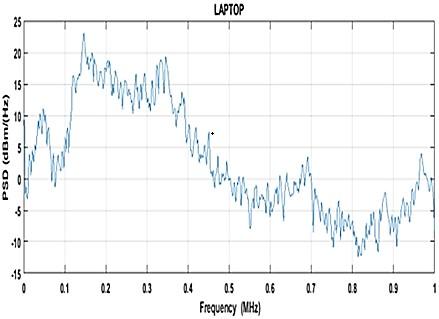
Figure 15 and 16 show the power spectral density of the computer and television (TV) set.
The integrand on the right side is identified as Power Spectral Density (PSD).
$G_{x}(f)=\lim _{T \rightarrow \infty} E\left(\left|F\left(\frac{X_{T}(t)}{T}\right)\right|^{2}\right)$ (12)
Average power of $\{X(t)\}=\int_{-\infty}^{\infty}(f) d f$ (13)
The noise power spectral density of the laptop varied between -2dBm (Hz) and 23dBm (Hz) and the high frequency noise process overlaid the low frequency noise process. The total noise spectral density of the computer (Samsung) has a maximum of 23dBm (Hz) at 0.13MHz. The noise spectral density of TV reaches a maximum level of 22dBm (Hz) at 0.15MHz. Between 0MHz and 0.4MHz the noise density spectral oscillate in the range from -2dBm (Hz) to 22dBm (Hz) in the frequency band from 0.5MHz to 0.9MHz.
As shown in Figure 17, the power spectral density of the noises produced by summations of all the appliances connected to the network were estimated using welch method.
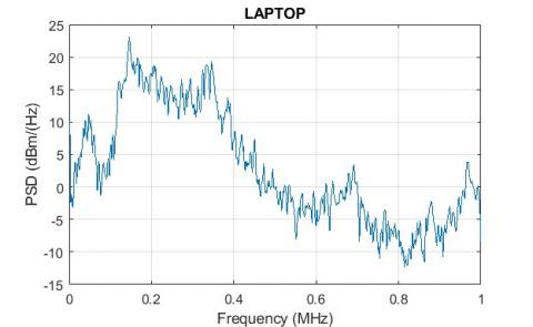
Figure 15. Noise density spectrum of a computer
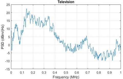
Figure 16. Noise density spectrum of a TV
Figure 17. Noise PSD summation
Different methods can be used for generating a noise PSD, among which are; periodogram and welch methods [18]. The periodogram is computed by taking Fourier Transform of the time and squaring the output. In comparison, both Welch and periodogram methods are good estimate of noise spectral density but, Welch method is better for good estimate of the noise spectral density and signal power at different frequencies. The noise PSD summation describes the variation of a signals power versus frequency. Background noise is generally characterized by a reasonably low power spectral density and this PSD tends to decrease as the frequency increases [17]. Our findings revealed that at low frequencies, the noise power is significantly higher and it is within the range of 0.1MHz to 0.35MHz. Hence, at higher frequencies, the noise power decreases. The results of this study indicate that transients that occur majorly are due to switching ON and OFF in different parts of electrical network and are the major causes of asynchronous impulsive noise. The durations of the impulsive noise ranges from few microseconds to milliseconds. The noise is sporadic and this can have severe impact on PLC communication systems. This however, calls for a very robust and accurate noise coding techniques and modulation schemes that can ease the effect of the PLC channel noise on the signal.
In this paper, we have been able to set up a measurement system design to capture the noise in time domain for a practical power line communication system. The behavioral statistics of impulsive noise in PLC base on its amplitude and durations of occurrence between impulses were presented. The findings observed in this study mirror those of the previous studies that have measured noise in PLC. We compared our results to that of literature elsewhere. The discrepancy could be attributed to electrical networks which differ significantly in structure, topology and physical characteristics. In comparison, the disparity with respect to durations and amplitude mean and standard deviation is quite significant. We concluded that the noise amplitude and durations are quite large. The amplitude of the noise signals can certainly be very large and this can be attributed to things like large transient, voltage spikes in equipment’s, lightning flashes, EMI on the network, topology and unknown characteristics of the power cables. Moreover, from the depicted noise PSD, it is clear that the laptop computer generates the worst noise disturbances, and this depends on the switching instances, which was unpredictable. Moreover, the noise in power line networks considered is very large, sporadic and this can have severe impact on PLC systems.
[1] Oluwafemi, I.B., Mneney, S.H. (2013). Review of space time coded orthogonal frequency division multiplexing systems for wireless communication. IETE Tech. Rev., 30(5): 417. https://doi.org/10.4103/0256-4602.123126
[2] Varma, M.K., Jaffery, Z.A., Ibraheem. (2019). Broadband power line communication: The channel and noise analysis for a power network. International Journal of Computer Network and Communication (IJCM), 11(1): 42-56. https://doi.org/10.5121/ijcnc.2019.11105
[3] Ali, S.S., Bhattacharya, A., Poddar, D.R. (2013). Modeling the noise for indoor power line channel. International Journal of Electronics Communication and Computer Engineering, 4(4): 1194-1198.
[4] Zhu, W. (2014). Power line communications over time-varying frequency-selective power line channels for smart home applications. Ph.D Dissertation. Electrical and Electronic Engineering Department. University of Liverpool, pp. 35-40.
[5] Zhu, W., Zhu, E., Lim, E., Huang, Y. (2017). State-of-art power line communications channel modelling. Procedia Computer Science, 17: 563-570. https://doi.org/10.1016/j.procs.2013.05.072
[6] Zhang, W., Luo, Z., Xiong, X. (2019). Impulse noise suppression based on power iterative ICA in power line communication. International Journal of Electronics and Telecommunications, 65(4): 651-656. https://doi.org/10.24425/ijet.2019.129824
[7] Canete, F.J., Cort, J.A., Dies, L., Entrambasaguas, J.T. (2003). Modeling and evaluation of the indoor power-line channel. IEEE Commun. Magazine, 41(4): 41-47. http://dx.doi.org/10.1109/mcom.2003.1193973
[8] Zimmermann, M., Dostert, K. (2002). A multipath model for the powerline channel. IEE Transactions on Communications, 50(4): 553-559. https://doi.org/10.1109/26.996069
[9] Parhi, K.K., Ayinala, M. (2014), Power spectral density computation. IEEE Transactions on Circuit and Systems, 61(1): 172-182. https://doi.org/10.1109/TCSI.2013.2264711
[10] Tlich, M., Chaouche, H., Zeddam, A., Pagani, P. (2009). Novel approach for PLC impulsive noise modelling. IEEE International Symposium, Dresden, Germany, pp. 20-25. https://doi.org/10.1109/ISPLC.2009.4913397
[11] Nyete, A. (2015), A Flexible statistical framework for the characterization and modelling of noise in power line communication. Ph.D Dissertation, University of Kwazulu-Natal, South Africa, pp. 33-42.
[12] Thomas, A., Modisa, M., Stephen, A. (2019). Measurements and statistical modeling for time behaviour of power line communication impulse noise. International Journal on Communications Antenna and Propagation, 9(4): 236. https://doi.org/10.15866/Irecap.vpi4.16094
[13] Mosalaosi, M., Afullo. T. (2014). Broadband analysis and characterization of noise for in-door power-line communication channels. Progress in Electromagnetic Research Symposium Proceedings, Guangzhou, no. Lc, pp. 719-722.
[14] Luis, D., Cort, A., (2002). Analysis of the indoor broadband power line. IEEE Transaction on Electromagnetic Compatibility, 52(4): 380.
[15] Hendrik, C., Vinck, J., Grove, H.M. (1996). Power line communications: An overview. IEEE AFRICON, 2: 13-16.
[16] Umehara, D., Hirata, S., Denno, S., Morihiro, Y. (2006). Modeling of impulse noise for indoor broadband power line communications. International Symposium on information Theory ant its Application, South Korea, pp. 195-199.
[17] Mosalaosi, M., Ramakrishna, P.V. (2014). Power line communication channel measurements and characterization. MSc Thesis, College of Agriculture, Engineering and Science, University of Kwazulu Natal, South Africa, pp. 26-39.
[18] Kees, J.T, Ernst, J.M., Headley, H., Beex, A.A. (2017). Robust blind spectral estimation in the presence of non-gaussian noise. MILCOM 2017 - 2017 IEEE Military Communications Conference (MILCOM), Baltimore, MD, USA, pp. 629-634. https://doi.org/10.1109/MILCOM.2017.8170868