Guglielmina Mutani* | Valeria Todeschi | Kaoru Matsuo
OPEN ACCESS
The phenomenon of overheating in urban areas is an increasingly important issue as far as the quality of life and public health are concerned. This paper proposes a simple model, integrated with a Geographic Information System (GIS) tool, that can be used to analyze the microclimate of outdoor spaces, considering the relationship between the air temperature and the characteristics of an urban environment. The Urban Heat Island (UHI) effect was analyzed by assessing parameters that describe the urban context, such as the density of the population and of the buildings, and the urban morphology. Remote sensing data and satellite images were used to evaluate the presence of vegetation and the type of surfaces in the urban space. Through the construction of linear regression models, the main variables of influence were identified for a typical summer day. It has been found, from the results, that the UHI effect decreases proportionally with the presence of vegetation and with higher values of the albedo of urban surfaces, as well as of the altitude and the distance from the sea. The UHI effect instead increases proportionally for higher values of the canyon height-to-width ratio, the building density and the Land Surface Temperature. These models can be used to analyse the outdoor thermal comfort and the livability of an urban territory.
Urban Heat Island (UHI), microclimate, linear regression models, urban environment, satellite images, GIS, urban morphology, NDVI, albedo
Global warming and rapid urbanization have significantly increased the urban heat island (UHI) effect, and UHI intensity has become a key aspect that should be considered to characterize the thermal environment of urban areas [1]. The UHI phenomenon is defined as a rise in temperature in dense city centers compared with the surrounding countryside [2]. In recent years, UHI phenomena caused by land cover changes and an increase in anthropogenic heat releases have been occurring in many cities throughout Japan [3] and in other countries; as a consequence, air temperatures have risen in urban areas. The UHI effect and global warming have caused adverse effects on human health and urban ecosystems, as well as uncomfortable outdoor environments and an increase in the energy consumed for space cooling. Therefore, in order to improve the livability and urban comfort of cities, it is necessary to identify mitigation measures, including improvements in land cover and ventilation, as well as reductions in anthropogenic heat releases [4]. The Japanese government has established guidelines concerning UHI mitigation. Five general actions have been identified: the reduction of anthropogenic heat emissions, the improvement of urban surfaces and structures, the improvement of lifestyles and the promotion of adaptation (The policy framework to reduce urban heat island effects, 2004, available at http://www.env.go.jp/en/air/heat/heatisland.pdf).
In previous researches, the authors investigated the microclimate of outdoor spaces in the Metropolitan City of Turin (Italy) considering the different outdoor air temperatures registered by several weather stations (WS). The air temperature variations were correlated with the built urban morphology, the solar exposure of urban spaces, the albedo coefficients of outdoor surfaces, the presence of vegetation and water (using the Normalized Difference Vegetation Index ‘NDVI’), the distance from the town center and the Land Surface Temperature (LST). A GIS-based method was used to calculate the parameters that influenced variations in the air temperature [5].
The aim of this work has been to present a methodology that can be used to mitigate Urban Heat Island (UHI) effects, and Hiroshima was selected as the case study. The method adopted to evaluate the air temperature variations and the UHI effect on the City of Hiroshima is presented in the first part of this work. Moreover, the data and the variables used to construct the models are indicated: satellite images (Landsat 7 and 8), WS data and their localization, and indicators used to implement the UHI models. The Hiroshima case study and the evaluation of its microclimate conditions in an urban context (air temperature, wind speed and wind direction) as well as the assessment of outdoor thermal comfort are dealt with in the second part using indexes based on linear equations. The results of the application of the models are also shown with the spatial distributions of the air temperature and maps obtained with the support of a GIS tool (ArcGIS 10.6).
The microclimate of outdoor spaces was investigated in a previous research pertaining to the Metropolitan City of Turin (Italy) considering different outdoor air temperatures registered by various WSs [5]. The UHI models presented in this work were then applied in the Hiroshima case study. The aim was to obtain a simple GIS-based model for the simulation of the hourly air temperature through the use of a linear regression.
Figure 1. Flowchart of the methodology
Figure 1 shows the methodology used to evaluate the outside air temperature. All the variables were identified on a building block territorial unit using a GIS tool (ArcGIS 10.6). The variables were then correlated with the outside air temperature, through the use of a linear regression model, in order to identify the main parameters of influence. More models were reported as functions of different numbers of variables. Finally, the hourly variation of the outside air temperature was evaluated and the territory was classified as: ‘mountain area’, ‘plain area near the sea’ and ‘plain area not near the sea’. This classification influences the air temperatures and their daily amplitude. The air temperature variations were correlated with the following variables, which were used to analyze the UHI phenomenon [6]: altitude (masl), distance from the sea (Dsea), albedo of the outdoor surfaces (ANIR), normalized difference vegetation index (NDVI), land surface temperature (LST), building coverage ratio (BCR), building density (BD), building height (BH) or relative height (H/Havg), canyon height-to-width ratio (H/W) and main orientation of the streets (MOS). These variables were calculated at a building block scale for each WS, considering all the blocks in a buffer area of 300 m from the WS. MOS was evaluated considering a variable that ranged from 0 to 1, with 0 corresponding to the North-South direction and 1 to the West-East direction. Satellite images (Landsat 7 and 8) were used to calculate the ANIR, LST and NDVI parameters, with reference to a typical summer day. The satellite images were chosen in the same period of weather measurements (from July 20th to September 23rd 2013) with no clouds the sky (less than 4 %). With the hourly distribution of air temperature, it was possible to define the typical summer day. The UHI models were defined by comparing the calculated air temperatures with the measured ones and then reducing the errors. An iterative procedure was performed on excel spreadsheets in order to reduce the errors between calculated and measured data, and to optimize the error (ε), the relative error (εr) and the relative absolute error (|εr|).
2.1 The air temperature model
The main variables of influence pertaining to the outside air temperature were identified considering the correlations between the variables and the outside air temperature. The linear regression models of the air temperature were set up considering all the variables or a limited number of variables. The linear regression model was created using 19th August 2013 at 1:49 a.m. (Eq. (1)) as the reference:
$T_{1: 49}=I+\alpha_{1} \cdot X_{1}+\alpha_{2} \cdot X_{2}+\ldots+\alpha_{n} \cdot X_{n}$ (1)
where, ‘I’ is the intercept; ‘αn’ are coefficients used to estimate the influence of variables X on the outdoor air temperature; ‘Xn’ are the independent variables.
The ‘min-max’ method (Eq. (2)) was introduced in order to normalize the variables and to evaluate the different weights of the variables on the air temperature:
$X_{N}=\frac{1}{X_{\max }-X_{\min }} \cdot X-\frac{X_{\min }}{X_{\max }-X_{\min }}$ (2)
Therefore, the normalized variables were dimensionless and varied from 0 to 1 (XN). The accuracy of the models was assessed with |εr| and εr.
2.2 The hourly air temperature model
The hourly trend of a typical summer day was analyzed, with Eqns. (3), (3.1), (3.2) and (3.3), as a function of the minimum, maximum and daily distribution of the air temperature. These values were mainly influenced by the altitude, the distance from the sea and the presence of vegetation and water (as characterized by the NDVI index). The territory was then classified as mountain area, plain area near the sea or plain area not near the sea.
An air temperature hourly-distribution factor, ‘f(t)’, was identified for the typical summer day and for each area to reduce |εr| and εr between the measured and calculated hourly air temperatures:
$T_{h}=T_{\min }+\Delta T^{\cdot} f(t)$ (3)
where,
$T_{\min }=I+\alpha_{A I t} \cdot A l t+\alpha_{D i s t} \cdot D i s t+\alpha_{N D V l} \cdot N D V I$ (3.1)
$\Delta T=I+\alpha_{A l t} \cdot A l t+\alpha_{D i s t} \cdot D i s t+\alpha_{N D V I} \cdot N D V I$ (3.2)
$f(t)=\frac{T_{h}-T_{\min }}{T_{\max }-T_{\min }}$ (3.3)
2.3 The thermal comfort indexes
The microclimate is affected by the local urban morphology [7] and several parameters, such as the H/W ratio, the sky view facto (SVF), the main orientation of the streets (MOS) or the albedo of outdoor surfaces, are used to describe the urban context, [8]. It has been found, from a literature review, that indexes used to assess comfort can be classified into three categories: energy balance models (i.e. Physiologically Equivalent Temperature ‘PET’; Predicted Mean Vote ‘PMV’; Perceived Temperature ‘PT’), empirical indices (i.e. Actual Sensation Vote ‘ASV’; Thermal Sensation Vote ‘TSV’) and indices based on linear equations (i.e. Apparent Temperature ‘AT’; Cooling Power Index ‘PE’; Wind Chill Temperature ‘WCT’) [9, 10, 11].
Among the various indicators for calculating thermal comfort, those that depend only on temperature Tair (°C), relative humidity RH (%), vapour pressure vp (hPa) and velocity v (m/s) of the outdoor air have been selected. In this work the following indicators were used with the relative correlations [9]:
$A T=-2.7+1.04 \cdot T_{a i r}+\frac{2 \cdot v p}{10}-0.65 \cdot v$ (4)
Discomfort Index ‘DI’ is used to quantify the effective temperature combining the effect of temperature, humidity and air movement on the sensation of heat or cold perceived by the human body:
$D I=T_{a i r}-0.55 \cdot(1-0.01 \cdot R H) \cdot\left(T_{a i r}-14.5\right)$ (5)
Normal Effective Temperature ‘NET’ is the effective temperature felt by the human organism for certain values of meteorological parameters such as air temperature, relative humidity of air, and wind speed:
$\begin{aligned} N E T=37 &-\frac{37-\tau_{\text {air }}}{0.68-0.0014 \cdot R H+\frac{1}{1.76+1.4 \cdot V^{-10.75}}}-0.29 \cdot T_{\text {air }} \\ &(1-0.01 \cdot R H) \end{aligned}$ (6)
Humidex ‘H’ was created to quantify and the degree of risk to the human body in the event of heat and excessive moisture (in cooling season); the simplified formula is the following:
$H=T_{a i r}+\frac{5}{9} \cdot(v p-10)$ (7)
Heat Index ‘HI’, also known as an apparent temperature, is the perceived temperature by the human body when relative humidity is combined with the air temperature:
$\begin{aligned} H I=& 8.784695+1.61139411 \cdot T_{a i r}+2.338549 \\ R H-0.14611605 \cdot T_{a i r} \cdot R H-1.2308094 \cdot 10^{-2} & . \\ T_{a i r}^{2}-1.6424828 \cdot 10^{-2} \cdot R H^{2}+2.211732 \cdot 10^{-3} \\ T_{a i r}^{2} \cdot R H+7.2546 \cdot 10^{-4} \cdot T_{a i r} \cdot R H^{2}-3.582 \\ 10^{-6} \cdot T_{s i r}^{2} \cdot R H^{2} \end{aligned}$ (8)
Relative stain index ‘RSI’ is used to describe the thermal comfort of a standard pedestrian under specific environmental conditions:
$R S I=\frac{\left(T_{a i r}-21\right)}{(58-v p)}$ (9)
Hiroshima is the capital of Hiroshima ken (prefecture) and it is located in the southwestern part of Honshu, in Japan. It has a rich topography with islands, the water of the Seto Inland Sea in the South and the Chugoku mountains in the North. Hiroshima had an estimated population of 1,195,327 in 2017 with a population density of 1,321 inh/km2 and a buildings density of 1.8 m3/m2 (quite low compared with European cities; for example, in Turin-IT these data are 6,917 inh/km2 and 4.5 m3/m2).
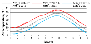
Hiroshima has a humid subtropical climate characterized by cool to mild winters and hot humid summers; like much of the rest of Japan, the warmest month of the year is August.
Figure 2 shows the average air temperature (Tair) of ‘Hiroshima WS’, which is located in the urban center of the city at an altitude of 3.7 m a.s.l. and BD of 6.7 m3/m2. The average annual Tair of Hiroshima, considering the last decade, is 16.51 °C, with lower values of 5.15 °C in January (minimum Tair is 1.72 °C) and higher values in August of 28.58 °C (maximum Tair is 32.91 °C). In this study, a typical summer day of 2013 was chosen, because the year 2013 was similar to the average trend of the last 10 years (average annual air temperature is 16.58 °C).
The typical summer day was chosen at August 19th 2013 because of the available satellite images with optimal visibility and low presence of clouds.
Figure 2. Air temperature of ‘Hiroshima WS’: the continuous lines show the average data from 2007 to 2017, while the dotted lines indicate the average data for 2013
3.1 Data collection
In this work, the data used to create the UHI models were organized with the support of a GIS tool (Table 1). The data refer to:
Table 1. Description of the data collection
|
Type of Data |
Reference |
Variables |
|
Satellite images |
Landsat 7 and 8 |
ANIR, NDVI, LST |
|
Building variables |
Municipal Technical Map |
m2, m3, BCR, BD, BH, H/W, MOS, blocks of building units |
|
Weather data |
7 municipal and 60 school weather stations |
Tair, RH, vp, v, winddirection |
|
Territorial characteristics |
Digital Elevation Model (DEM) at 10 m |
masl |
|
Municipal Technical Map |
Land cover (type of users) |
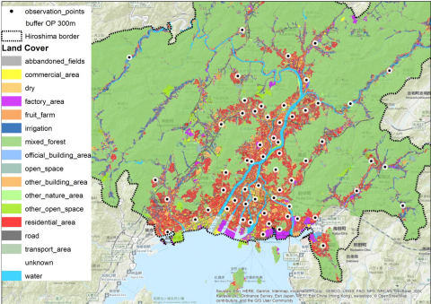
Figure 3. Land Cover of Hiroshima and localization of the weather stations
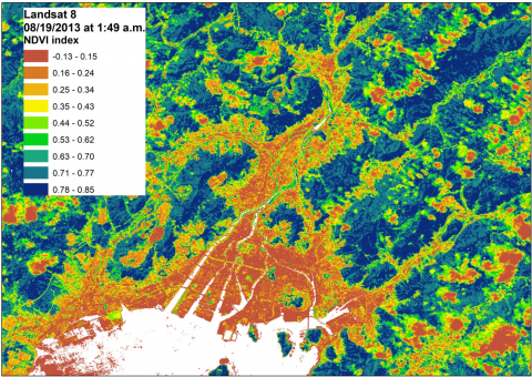
Figure 4. NDVI evaluated with the support of ArcGIS from Landsat 8 satellite images for August 19th 2013 at 1:49 a.m
Figure 3 and 4 show an example of the available GIS database. Figure 3 classifies the territory on the basis of the presence of water/vegetation and the built-up areas considering the land cover for residential, commercial, industrial and tertiary use. Figure 4 shows the NDVI index evaluated through the use of satellite images, where the distribution of vegetation, water and built-up areas is highlighted; it is possible to observe that, in the urban context, there are some green areas that may influence the microclimate and the UHI effect (i.e. -1=water, 0=bare soil, 1=dense green vegetation).
3.2 Classification of the weather stations
Mitigation measures depend on different urban variables (microclimate, altitude, urban density, distance from the center of the city), and it is necessary to also consider the effect of sea proximity and breezes [12] for coastal cities. The sea breezes in Hiroshima affect the local climate in coastal urban areas as much as the ground surface condition does. Therefore, in order to set up the UHI models, the WSs were classified considering their altitude and their distance from the sea. The models were created using weather data, and distinguishing between temperature stations and wind stations. The temperature distribution was analyzed considering 60 observation points, which involved installing 60 temperature sensors with instrumented screens outside schools. The observation period was from 20th July 2013 to September 23rd 2013, and an observation interval of 1 hour was introduced. The wind direction and wind speed were analyzed using seven municipal weather stations: the hourly wind direction (0 from the North direction) and hourly speed data were already known for the same period. The temperature stations were classified into three clusters considering the altitude and the distance from the sea (Figure 5):
Figure 5. LST from Landsat 8 satellite images (August 19th 2013 at 1:49 a.m.) at a building block scale and localization of the WSs (wind stations and temperature stations in mountain and plain areas near/not near the sea)
In order to evaluate the influence of the altitude on the air temperature, the correlation factor ‘d’ (in °C/m) was calculated by means of Eq. (10):
$T_{z}=T_{z, r e a l}-\left(z-z_{r e a l}\right) \cdot d$ (10)
In the mountain area, considering the greater differences in altitude, the temperature-altitude coefficient ‘d’ was estimated to have an average value of 166.1 °C/m.
The air temperature characteristics for the above mentioned three areas are reported in Table 2. It is possible to observe that: the average air temperature in the mountains is lower than that in the plain areas because the temperature is influenced by the altitude (with also a higher standard deviation); the air temperature amplitude (∆T) is lower near the sea, as a result of the mitigating effect of the large mass of water (at an altitude of less than 11 m a.s.l.); the average air temperatures are similar for the 3 areas.
Table 2. Description of the weather data
|
WSs |
Air Temperatures |
||||
|
ΔT |
Tmin |
Tmax |
Tavg |
St.Dev. |
|
|
Plain near the sea |
8.5 |
27.1 |
35.6 |
31.0 |
0.4 |
|
Plain not near the sea |
11.0 |
25.7 |
36.8 |
31.0 |
0.4 |
|
Mountain |
11.7 |
24.3 |
35.9 |
29.7 |
0.7 |
Table 3. Description of the weather data
|
WS ID |
Dsea [m] |
masl [m a.s.l.] |
Tavg [°C] |
NDVI [-1;1] |
ANIR [0;1] |
LST [°C] |
MOS [0;1] |
BCR [m2/m2] |
BD [m3/m2] |
BH [m] |
H/Havg [-] |
H/W [-] |
|
Mountain Weather Stations (n. 17) |
||||||||||||
|
3 |
5,680 |
126 |
30.72 |
0.49 |
0.24 |
24.67 |
0.35 |
0.08 |
0.50 |
6.16 |
1.02 |
0.13 |
|
7 |
6,233 |
142 |
29.98 |
0.43 |
0.25 |
25.03 |
0.20 |
0.30 |
1.82 |
6.26 |
1.05 |
0.23 |
|
8 |
21,163 |
99 |
28.72 |
0.49 |
0.25 |
24.66 |
||||||
|
10 |
16,326 |
236 |
29.32 |
0.39 |
0.25 |
25.25 |
0.62 |
0.19 |
1.07 |
5.97 |
1.03 |
0.15 |
|
11 |
11,015 |
80 |
29.42 |
0.42 |
0.23 |
24.87 |
0.77 |
0.11 |
0.62 |
6.58 |
0.92 |
0.37 |
|
12 |
18,685 |
82 |
28.68 |
0.50 |
0.19 |
23.56 |
||||||
|
14 |
18,233 |
60 |
29.87 |
0.39 |
0.21 |
25.39 |
0.51 |
0.17 |
0.92 |
5.87 |
1.07 |
0.13 |
|
16 |
9,919 |
179 |
29.20 |
|
|
|||||||
|
25 |
10,318 |
77 |
29.94 |
0.51 |
0.25 |
23.92 |
0.48 |
0.16 |
0.87 |
5.28 |
1.02 |
0.10 |
|
26 |
9,748 |
152 |
29.46 |
0.49 |
0.29 |
26.03 |
0.48 |
0.14 |
0.74 |
5.66 |
1.00 |
0.14 |
|
36 |
18,808 |
170 |
28.43 |
0.63 |
0.25 |
22.73 |
||||||
|
37 |
14,026 |
126 |
30.14 |
0.47 |
0.28 |
23.59 |
0.35 |
0.24 |
1.72 |
7.08 |
1.10 |
0.20 |
|
44 |
6,950 |
134 |
30.48 |
0.59 |
0.27 |
23.76 |
0.49 |
0.19 |
1.97 |
13.79 |
1.82 |
0.19 |
|
48 |
13,672 |
148 |
30.43 |
0.33 |
0.25 |
26.47 |
0.56 |
0.24 |
1.49 |
6.41 |
1.06 |
0.18 |
|
49 |
9,265 |
150 |
29.58 |
0.36 |
0.27 |
25.21 |
0.46 |
0.27 |
1.53 |
5.77 |
1.01 |
0.20 |
|
50 |
7,109 |
104 |
30.73 |
|
|
|
0.55 |
0.26 |
1.39 |
5.59 |
1.06 |
0.18 |
|
61 |
19,473 |
63 |
30.28 |
0.38 |
0.22 |
25.34 |
0.51 |
0.22 |
1.19 |
5.76 |
1.07 |
0.14 |
|
Plain Weather Stations near the sea (n. 24) |
||||||||||||
|
1 |
1,131 |
3 |
30.27 |
0.20 |
0.21 |
26.58 |
0.48 |
0.30 |
2.31 |
9.14 |
1.31 |
0.21 |
|
2 |
3,711 |
2 |
30.93 |
0.15 |
0.19 |
27.27 |
0.38 |
0.27 |
1.97 |
8.74 |
1.28 |
0.24 |
|
4 |
274 |
3 |
30.34 |
0.17 |
0.23 |
26.24 |
0.28 |
0.34 |
2.60 |
9.07 |
1.40 |
0.23 |
|
5 |
4,440 |
31 |
30.74 |
0.41 |
0.24 |
25.68 |
0.55 |
0.26 |
1.56 |
6.63 |
1.18 |
0.18 |
|
6 |
3,393 |
8 |
30.55 |
0.23 |
0.22 |
26.25 |
0.60 |
0.30 |
1.76 |
6.46 |
1.13 |
0.21 |
|
9 |
1,917 |
9 |
30.67 |
0.25 |
0.21 |
26.38 |
0.43 |
0.35 |
2.15 |
6.69 |
1.15 |
0.27 |
|
21 |
1,740 |
17 |
30.62 |
0.34 |
0.23 |
26.25 |
0.57 |
0.27 |
1.49 |
5.91 |
1.10 |
0.19 |
|
22 |
1,444 |
4 |
31.21 |
0.17 |
0.19 |
27.59 |
0.37 |
0.35 |
2.01 |
6.38 |
1.13 |
0.23 |
|
23 |
2,001 |
3 |
31.38 |
0.17 |
0.19 |
26.91 |
0.40 |
0.32 |
2.25 |
8.99 |
1.42 |
0.23 |
|
28 |
2,990 |
4 |
31.20 |
0.06 |
0.17 |
25.90 |
0.37 |
0.21 |
1.84 |
11.59 |
1.81 |
0.17 |
|
30 |
611 |
3 |
30.60 |
0.14 |
0.22 |
27.54 |
0.44 |
0.31 |
2.35 |
8.73 |
1.28 |
0.28 |
|
34 |
1,397 |
5 |
31.27 |
0.19 |
0.21 |
27.18 |
0.43 |
0.33 |
1.96 |
6.47 |
1.14 |
0.22 |
|
38 |
4,279 |
3 |
31.51 |
0.10 |
0.18 |
26.03 |
0.42 |
0.39 |
6.84 |
21.38 |
1.52 |
0.53 |
|
43 |
3,988 |
3 |
31.74 |
0.11 |
0.17 |
26.76 |
0.48 |
0.33 |
2.80 |
10.05 |
1.36 |
0.31 |
|
45 |
876 |
14 |
31.13 |
0.31 |
0.25 |
26.61 |
0.35 |
0.22 |
1.64 |
7.67 |
1.30 |
0.15 |
|
47 |
4,853 |
8 |
31.04 |
0.20 |
0.20 |
26.01 |
0.40 |
0.31 |
2.32 |
9.31 |
1.35 |
0.26 |
|
51 |
2,541 |
4 |
31.59 |
0.13 |
0.20 |
27.29 |
0.47 |
0.33 |
2.37 |
9.04 |
1.26 |
0.29 |
|
52 |
2,627 |
2 |
30.92 |
0.16 |
0.21 |
26.99 |
0.48 |
0.25 |
1.93 |
9.76 |
1.50 |
0.19 |
|
53 |
1,342 |
1 |
30.92 |
0.19 |
0.22 |
27.52 |
0.53 |
0.30 |
2.08 |
7.84 |
1.23 |
0.25 |
|
54 |
5,217 |
3 |
31.07 |
0.11 |
0.16 |
26.28 |
0.38 |
0.34 |
3.51 |
13.75 |
1.56 |
0.34 |
|
55 |
3,811 |
2 |
31.18 |
0.11 |
0.17 |
25.46 |
0.54 |
0.30 |
3.54 |
15.28 |
1.61 |
0.33 |
|
56 |
1,835 |
3 |
30.98 |
0.01 |
0.16 |
25.09 |
0.45 |
0.35 |
2.45 |
7.83 |
1.18 |
0.32 |
|
57 |
5,495 |
4 |
31.09 |
0.17 |
0.21 |
26.35 |
0.36 |
0.30 |
3.07 |
12.45 |
1.38 |
0.29 |
|
58 |
2,239 |
5 |
30.57 |
0.07 |
0.17 |
26.04 |
0.43 |
0.32 |
2.32 |
8.11 |
1.17 |
0.30 |
|
Plain Weather Stations not near the sea (n. 18) |
||||||||||||
|
13 |
15,593 |
16 |
31.21 |
0.28 |
0.23 |
26.03 |
0.46 |
0.15 |
0.95 |
7.89 |
1.27 |
0.13 |
|
15 |
12,399 |
41 |
30.60 |
0.31 |
0.23 |
24.96 |
0.43 |
0.19 |
1.23 |
6.66 |
1.07 |
0.16 |
|
17 |
13,868 |
57 |
30.21 |
0.62 |
0.26 |
23.41 |
||||||
|
18 |
8,101 |
25 |
30.28 |
0.39 |
0.25 |
25.58 |
0.51 |
0.29 |
1.72 |
6.27 |
1.09 |
0.23 |
|
19 |
13,205 |
26 |
30.54 |
0.30 |
0.17 |
24.76 |
0.46 |
0.16 |
0.89 |
5.70 |
1.05 |
0.13 |
|
24 |
9,650 |
8 |
31.29 |
0.17 |
0.21 |
27.42 |
0.51 |
0.30 |
1.90 |
7.24 |
1.18 |
0.21 |
|
27 |
8,424 |
10 |
31.13 |
0.17 |
0.20 |
26.54 |
0.40 |
0.33 |
2.25 |
7.55 |
1.21 |
0.24 |
|
29 |
6,437 |
34 |
30.25 |
0.38 |
0.26 |
25.96 |
0.43 |
0.22 |
1.20 |
5.95 |
1.09 |
0.16 |
|
32 |
12,405 |
19 |
31.16 |
0.28 |
0.23 |
26.62 |
0.53 |
0.29 |
2.17 |
8.08 |
1.23 |
0.21 |
|
33 |
9,567 |
7 |
31.55 |
0.28 |
0.24 |
26.59 |
0.58 |
0.17 |
1.03 |
6.27 |
1.11 |
0.15 |
|
35 |
13,216 |
43 |
30.85 |
0.38 |
0.22 |
25.71 |
0.45 |
0.24 |
1.41 |
6.31 |
1.09 |
0.19 |
|
39 |
13,159 |
19 |
31.28 |
0.27 |
0.22 |
26.60 |
0.46 |
0.21 |
1.31 |
6.43 |
1.12 |
0.17 |
|
40 |
11,853 |
44 |
31.18 |
0.26 |
0.21 |
26.76 |
0.45 |
0.30 |
1.79 |
6.05 |
1.03 |
0.21 |
|
41 |
8,381 |
9 |
31.40 |
0.21 |
0.19 |
26.02 |
0.44 |
0.31 |
2.27 |
8.57 |
1.36 |
0.23 |
|
42 |
11,493 |
9 |
31.30 |
0.22 |
0.22 |
27.37 |
0.48 |
0.22 |
1.35 |
6.68 |
1.14 |
0.18 |
|
46 |
12,680 |
25 |
31.12 |
0.32 |
0.21 |
26.06 |
0.32 |
0.20 |
1.30 |
7.26 |
1.21 |
0.16 |
|
59 |
10,136 |
8 |
31.33 |
0.23 |
0.21 |
27.13 |
0.52 |
0.24 |
1.77 |
8.15 |
1.26 |
0.22 |
|
60 |
8,113 |
9 |
30.74 |
0.24 |
0.21 |
26.38 |
0.53 |
0.30 |
2.02 |
7.45 |
1.21 |
0.24 |
Table 3 shows the distance from the sea, the altitude, the temperature data, which refer to August 19th 2013, the NDVI, Albedo ANIR and LST (in Figure 5), which refer to satellite images and urban variables for each WS. The variables were calculated at a building block scale for each WS and an average value was identified considering a circular buffer area of 300 m around the WS. The urban variables were not calculated for 5 WSs, either because the information pertaining to the building blocks (WS ‘12’ and ‘17’) was missing or because the weather stations were located in non-built up areas (WS ‘8’, ‘16’ and ‘36’) or in cloudy zones (WS ‘16’ and ‘50’) in the satellite images.
The urban climate of Hiroshima was analyzed through the use of 60 WSs of elementary schools for the year 2013 from July 20th, to September 23rd. Moreover, the wind characteristics were investigated considering the data from 7 municipal WSs that were available for the same period. The WSs were classified as mountain, plain near the sea or plain not near the sea WSs. The evaluation of the WS data showed that, for the 60 analyzed WSs, the minimum air temperature almost always occurred at 6 a.m. (97 % of the WSs), whereas the maximum temperature was measured at 3 p.m. (57 % of the WSs; 92 % of the WSs, but also considering 2 p.m.).
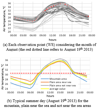
Figure 6a shows the average hourly temperature value for each observation point considering the month of August, where the red dotted line refers to August 19th 2013. In this work, August 19th in 2013 was chosen as a typical summer day because the daily trend was regular and the temperatures were higher than 90 % of the data pertaining to August. This typical day corresponds to a hot summer day (where the hottest days were excluded).
Figure 6. WS data: Hourly outdoor air temperatures
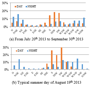
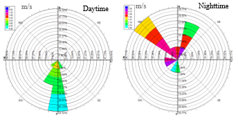
The wind data were analyzed considering the daytime and nighttime of August 19th 2013; daytime is from 9 a.m. to 7 p.m. and nighttime is from 8 p.m. to 8 a.m. (Figure 6b). The hourly wind direction and hourly wind speed were then explored considering 7 municipal wind stations, and the average hourly values from July 20th, 2013 to September 30th, 2013 (Figure 7a) were compared with the hourly values of August 19th 2013 (Figure 7b). Figure 7 show the direction and wind speed on 19th August 2013 as measured at municipal WS7 (localized in a mountain area), distinguishing between the daytime and the nighttime (Figure 8); the main wind direction during the daytime is Southern, as are the typical descending mountain breezes, with an average speed value of 3.7 m/s (higher than the nighttime value of 1.3 m/s); the main wind direction in the nighttime is instead Northern, that is, in the opposite direction to the daytime one, due to the presence of the sea and the orientation of the mountains with ascending valley breezes.
Figure 7. WS data: Wind directions frequency
Figure 8. Wind rose diagram
The results shown below are divided into 4 sections. The first part is dedicated to the linear regression model used to create the air temperature model for the considered typical summer day (August 19th 2013). The results of the hourly air temperature distribution model are presented in the second part, where the weather stations located in the mountains area, plain area not near the sea and plain area near the sea are distinguished. In the third part, assessments of the urban heat island intensity were made using the UHI-driven indicators (Q1 and Q2) and land-cover-driven indicators (Q3) [13]; the heatwaves and cold waves for the years 2007 and 2013 were also analyzed. Outdoor thermal comfort indexes have been calculated in the last section comparing the results on seven weather stations.
4.1 The air temperature model
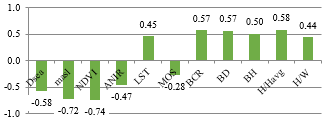
In order to identify the main variables of influence on the air temperature, the correlations between the variables and air temperature were evaluated (Figure 9). The altitude shows a negative correlation because the air temperature decreases as the altitude increases. The presence of vegetation and water also reduces the air temperature and NDVI therefore has a negative correlation, while positive correlations can be observed for BD, BCR, H/Havg and H/W.
Only variables that were not dependent on each other were used for the higher correlation factor. As BD and BCR are dependent variables, only BCR was used for the model; BH and H/Havg are also dependent, so only H/Havg was used for the model. The linear regression models of the air temperature are presented hereafter, where models with non-normalized variables are distinguished (Figure 10a): a linear regression model with all the non-normalized variables (Eq. 11); a linear regression model with the non-normalized variables but without LST (Eq. 12); and with normalized variables (Figure 10b): a linear regression model with all the normalized variables (Eq. 13); a linear regression model with the normalized variables but without LST (Eq. 14); a linear regression model with the normalized variables but without LST and NDVI (Eq. 15); a linear regression model with the normalized variables but without ANIR and LST (Eq. 16).
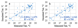
The best results, with the highest R2 coefficient of determination, were provided by Eq. 11 (all the non-normalized variables) and Eqns. 13 and 14 (all the normalized variables and all the normalized variables without LST). Table 4 reports the R2 values that show to what extent the variations in air temperature can be explained, by the regression model, as functions of the selected variables (Eqns. 12 and 14(Eqns. 12 and 14 without LST, Eq. 15 without LST and NDVI, and Eq. 16 without LST and ANIR).
The measured value of the relative error |εr|, which is the ratio of the absolute error, between the measured and calculated values of the air temperatures, was used to describes the accuracy of the models; low values can be observed for all the linear regression models and they tend to increase slightly when some variables, such as LST and NDVI, are excluded. Moreover, NDVI and ANIR are dependent variables, with a correlation coefficient of 0.76, and the weight of the variables should therefore be negative in the models, but the ANIR tends to be positive due to the presence of the NDVI (compensatory effect); in addition, for this case study, ANIR is quite constant, with an average value of 0.22 and a low standard deviation of 0.04.
The models were then applied to the Hiroshima territory through the use of the GIS tool. Figure 11 shows the air temperature simulated for August 19th 2013 at 1:49 a.m. using the model with all the normalized variables (Eq. 13). The air temperature is higher in urban areas than in the peripheral plain and mountain areas, where the temperature is mitigated by the altitude, the presence of vegetation and a lower buildings density.
Figure 9. Correlations between the variables and the air temperature
Figure 10. Air temperature models with (a) all the non-normalized variables and (b) all the normalized variables
Table 4. Eqns. 11-16: Coefficients, relative error |εr| and coefficient of determination R2 for air temperature models
|
Eq. |
(11) |
(12) |
(13) |
(14) |
(15) |
(16) |
|
I |
21 |
24 |
27 |
27 |
27 |
28 |
|
αD,sea |
0.000021 |
0.000012 |
-0.015 |
-0.015 |
-0.015 |
-0.015 |
|
α m,asl |
-0.01 |
-0.01 |
-2.13 |
-2.10 |
-2.42 |
-1.52 |
|
αNDVI |
-4.69 |
-6.43 |
-2.71 |
-3.24 |
- |
-1.91 |
|
αA,NIR |
11.33 |
13.56 |
1.54 |
1.82 |
-0.15 |
- |
|
αLST |
0.11 |
- |
0.39 |
- |
- |
- |
|
αMOS |
0.04 |
0.04 |
0.04 |
0.35 |
0.04 |
0.04 |
|
αBCR |
5.79 |
5.30 |
1.53 |
1.63 |
2.64 |
1.93 |
|
αH/Havg |
1.62 |
1.40 |
1.71 |
1.62 |
1.64 |
1.55 |
|
αH/W |
-0.19 |
-0.35 |
-0.34 |
-0.36 |
-0.76 |
-0.71 |
|
|εr|avg |
0.01 |
0.02 |
0.01 |
0.02 |
0.02 |
0.02 |
|
R2 |
0.78 |
0.77 |
0.79 |
0.78 |
0.73 |
0.75 |
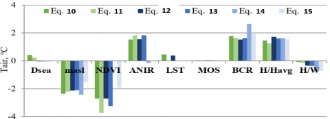
The range of variability of the different variables multiplied by the relative coefficients α is indicated in Figure 12. The main variables of influence (the non-normalized variables are in green, while the normalized variables are in blue) are: the altitude, the presence of vegetation, the characteristics of the outdoor surfaces (ANIR), the buildings density (BCR) and the relative building height (H/Havg). LST is present in two equations (Eq. 11 and 13); the ANIR coefficient becomes negative when NDVI is not included in the model (Eq. 15). The distance from the sea and the altitude are uncontrollable variables, and in order to improve the microclimatic conditions and, to mitigate the air temperature, it is therefore necessary to intervene on the other variables. For example, in newly built areas (where there is an increase in BCR and H/Havg, and consequently an increase in air temperature), the share of green areas can be improved (NDVI is inversely proportional to the air temperature) to compensate for the UHI effect. Eqns. 15 and 16 confirm the correlation between ANIR and NDVI; NDVI in Eq. 15 is inversely proportional to Tair, and the same relationship may be observed for ANIR in Eq. 16 without NDVI.
Figure 11. Air temperature model with all the normalized variables (Eq. 11)
Figure 12. Correlations between the variables and the air temperature
4.2 The hourly air temperature model
The outside air temperature was simulated using the equations reported in Table 5, in which the intercept ‘I’ and the weight coefficient of the ‘α’ variables (distance from the sea, altitude and presence of vegetation and water) are indicated: Eq. 17 refers to the whole territory; Eq. 18 refers to the mountain areas; Eq. 19 refers to the plain areas near the sea; Eq. 20 refers to the plain areas not near the sea.
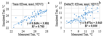
Figure 13 show the equations used to evaluate the daily minimum air temperature, Tmin, and the daily amplitude of the air temperature, Delta (t), for a hot summer day. The hourly air temperatures were then simulated, using Eq. 3, for a typical hot summer day (August 19th 2013). In these models, the relative error |εr| is higher and the coefficient of determination R2 is lower than in the other models, because Tair does not only depend on these variables; consequently, there is a greater dispersion of data from the average value (this trend is more evident in the case of the Delta (t) which has an average |εr| of 10.8 %).
Figure 13. Equations used to evaluate the: (a) minimum Tmin and (b) amplitude Delta(T) of the air temperature
Table 5. Eqns. 17-20: Coefficients, relative errors |εr| and coefficients of determination R2 for the hourly air temperature model
|
Eq. |
(17) |
(18) |
(19) |
(20) |
|
|
Tmin |
I |
28.4 |
27.2 |
27.9 |
28.5 |
|
αD,sea |
-0.00009 |
-0.0001 |
0.00006 |
-0.00009 |
|
|
αm,asl |
-0.009 |
-0.003 |
0.036 |
-0.022 |
|
|
αNDVI |
-4.45 |
-2.97 |
-5.44 |
-3.92 |
|
|
∆T |
I |
6.41 |
9.69 |
6.1 |
5.82 |
|
αD,sea |
0.00022 |
0.00005 |
0.0004 |
0.00025 |
|
|
αm,asl |
-0.002 |
0.005 |
-0.004 |
0.004 |
|
|
αNDVI |
6.05 |
0.5 |
5.55 |
7.64 |
|
|
|ε|avg |
2.20 % |
2.80 % |
2.00 % |
1.50 % |
|
|
Area |
Global |
Mountain |
Plain near |
Plain not-near |
|
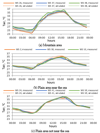
Figure 14. Distribution of the hourly air temperature for August 19th 2013
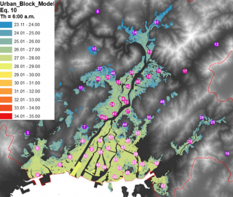
Figure 15. Application of the hourly air temperature model for 6 a.m. at a building block scale (Eq. 12)
Figure 16. Application of the hourly air temperature model for 3 p.m. at a building block scale (Eq. 12)
4.3 The UHI-driven and land-cover-driven indicators
The UHI intensity (UHII) is an indicator that can be used to measure the hourly and daily amplitude and temperature gradient of the air between the urban and the surrounding rural areas. Two types of indicators can be used to evaluate the different microclimate conditions: a UHI-driven type (Q1 and Q2) and a land-cover-driven type (Q3) [13]:
Q1. The ‘magnitude’ of the UHI-driven indicator is equal to the maximum temperature minus the average daily air temperature, where daytime is distinguished from nighttime;
Q2. The ‘range’ of the UHI-driven indicator is equal to the difference between the maximum and the minimum daily air temperatures, and daytime is distinguished from nighttime;
Q3. The ‘urban-rural’ land cover-driven indicator, which describes the difference between the hourly air temperatures in the urban and surrounding areas.
These three indicators were calculated with the hourly data for the years 2007 and 2013 for two municipal WSs: WS 7 (at altitude of 26.7 m a.s.l.), which is located in the surrounding rural area and WS 3 (at altitude of 5.8 m a.s.l.), which is located in an urban area (Figure 5).
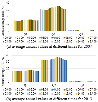
Figure 17 shows the trends of the indicators for the years 2007 and 2013 considering the annual average quantitative values of UHI intensity at different times. It is possible to see that the values of Q1 and Q2 remain almost stable and the values decrease from midnight to 6 a.m., then there is a slight increase and the UHI effect tends to decrease after 4 p.m. (this trend is similar for both years); Q3 decreases during the day and tends to increase after 6 p.m.
Figure 17. The UHI-driven and land-cover-driven indicators
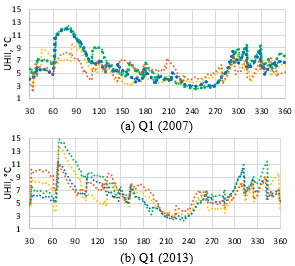
Figure 18, Figure 19 and 20 show the moving average times series of the previous 30 days of the UHII values at 0 a.m., 6 a.m., 10 a.m. and 2 p.m. Different trends may be observed: Q1 and Q2 have lower daytime values in winter than nighttime values, while the daytime values in summer are higher than the nighttime values. Moreover, the land-cover-driven indicator Q3 has higher values in winter due to the higher thermal excursion that occurs during the night (this effect is due to lower air temperatures); Q3 is higher in the daytime in summer due to higher solar irradiation. The urban station always has smaller values than the suburban station because Tair is influenced by the urban density, with higher air temperature values. In fact, WS 3 has a BCR of 0.33 m2/m2 and a BD of 3.05 m3/m2, which are higher than WS 7 (BCR = 0.23 m2/m2 and BD = 1.64 m3/m2).
The heatwaves and cold-waves were evaluated for the years 2007 and 2013 using the same weather station data (WS 3 and WS 7). The heatwaves were considered as events with temperatures over the 97.5th percentile and cold-waves as events with temperature under the 2.5th percentile [14]. In 2007 and 2013, there were 10 hot days a year in Hiroshima, with an average air temperature of 30.43 °C in 2007 and 31.39 °C in 2013, with heatwaves with higher air temperature than 29.8 °C for the year 2007 and 31.01 °C for the year 2013. Moreover, there were 9 cold days a year with an average air temperature of 3.36 °C in 2007 and 1.37 °C in 2013, with cold-waves with a lower air temperature than 4.24 °C for the year 2007 and 2.48 °C for the year 2013.
Figure 18. The Q1: 30 UHI-driven indicator for the moving average times series of UHI intensity at 0 a.m. (in blue), 6 a.m. (in green), 10 a.m. (in yellow) and 2 p.m. (in orange)
Figure 19. The Q2:30 UHI-driven indicator for the moving average times series of UHI intensity at time 0 a.m. (in blue), 6 a.m. (in green), 10 a.m. (in yellow) and 2 p.m. (in orange)
Figure 20. The Q3: 30 UHI-driven indicator for the moving average times series of UHI intensity at time 0 a.m. (in blue), 6 a.m. (in green), 10 a.m. (in yellow) and 2 p.m. (in orange)
Figure 21 shows the average hourly UHI variability during the summer months (June-August) for Hiroshima. The data for the summer months for the years 2007 and 2013 were used to analyze the UHI variability trend. The shaded area in Figure 21 represents the average hourly standard deviation, while the dashed lines with the sun and the moon symbols represent the approximate local sunrise (5 a.m.) and sunset (7 p.m.) times. The UHII increases between the hours 3 p.m. to 1 a.m. and decreases during the period 3 a.m. to 3 p.m.; the highest UHI value is 1.5 °C and it may be observed at 1 a.m. (average value for the years 2007 and 2013). This trend is due to the influence of coastal winds and it is similar to that of the City of Seattle, which is located near the coast [1]. In fact, wind effects, in addition to the surface characteristics, play a crucial role in influencing the UHII; as the wind speed increases, the volume of relatively cooler air arriving from the surrounding rural areas reduces the urban air temperature. These air circulations play a crucial role in reducing the horizontal temperature gradient between the urban and rural areas [1].
Figure 21. Mean daily variability of the UHII for summer months (June-August)
4.4 The thermal comfort assessment
Six indexes were used to analyze outdoor thermal comfort in summertime [9] based on linear equations depending on the available three climate variables: air temperature, relative humidity and velocity. The outdoor thermal conditions were assessed using the data from seven weather stations considering the typical summer day with hourly intervals. In general, it is possible to observe that the low distance from the sea (WS1, WS4), the high altitude (WS7), the presence of the wind (WS1, WS4, WS5, WS6 and WS7), and of green areas (WS5) significantly increase the outdoor thermal comfort.
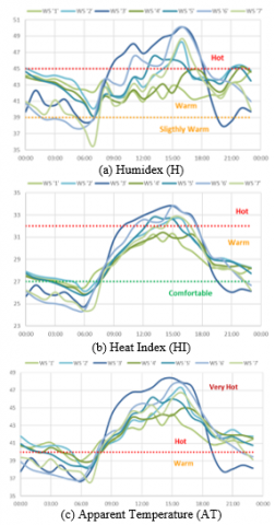
Figure 22 shows some examples of the hourly results for three thermal comfort indexes: Apparent Temperature (AT), Humidex (H) and Heat Index (HI). Only for WS1 and WS4 warm thermal comfort conditions were recorded for H and HI indexes; these results are mainly due to the proximity to the sea, and to the presence of the wind. The worst thermal comfort conditions are observed for WS3 and WS6; in WS3 there was no wind and WS6 low green areas and high buildings density. Thermal comfort in summertime is correlated to the type of urban environment but also by the presence of wind.
Figure 22. Hourly trends of thermal comfort indicators
In Hiroshima, the issue of the urban heat island phenomenon has been reported to engender high temperatures. Therefore, urban planning that incorporates the mitigation of the UHI phenomenon is needed.
This work has shown that the UHI effects in Hiroshima are influenced by the built-up areas, the presence of water and vegetation, the speed and direction of the wind, the distance from the sea and the altitude. The hourly air temperature models had the objective of establishing what the main variables that influence the UHI effect are and of understanding how, through the compensative method, it would be possible to improve urban comfort and the local microclimatic conditions. For example, an increase of 20% in NDVI determines an average decrease in air temperature of about 0.2 °C. The reliability of the models depends on the amount of available data and their quality. In these UHI models, the errors are also influenced by the variability of the indicators; for example, in Hiroshima, the albedo values are very low, with a standard deviation of 0.04; moreover, the NDVI index has only positive values. In addition, the choice of a typical summer day was conditioned by the availability of satellite images with a cloud coverage above 4%.
The UHI indicators were used to describe the UHI intensity, and the results show that: the trend of UHI-driven indicators (Q1 and Q2) is always positive and constant; the land-cover-driven indicator (Q3) shows higher air temperatures in urban areas than in suburban areas, due to a concentration of human activities. From 2007 to 2013, the average air temperature of the heatwaves increased from 30.4 to 31.4 °C and the average air temperature of the cold-waves decreased from 3.4 to 1.4 °C.
Moreover, the thermal comfort analysis confirmed the important role of urban variables besides climate conditions (i.e. the presence of the wind).
The planning of urban areas for future developments could be improved through the application of these models to increase the livability of a territory; besides, weather conditions strongly influence the use of energy [15], especially for space heating and cooling [16], and then climate mitigation measures can also cause a lower impact on the environment.
G. Mutani and V. Todeschi contributed equally to definition and analysis on the UHI and to the writing of manuscript. K. Matsuo has provided the data of Hiroshima’s case study.
[1] Ramamurthy, P., Sangobanwo, M. (2016). Inter-annual variability in urban heat island intensity over 10 major cities in the United States. Sustainable Cities and Society, 26: 65-75. http://doi.org/10.1016/j.scs.2016.05.012
[2] Nakata-Osaki, C.M., Souza, L.C.L., Rodrigues, D.S. (2018). THIS – tool for heat island simulation: A GIS extension model to calculate MARK urban heat island intensity based on urban geometry. Computers, Environment and Urban Systems, 67: 157-168. http://doi.org/10.1016/j.compenvurbsys.2017.09.007
[3] Ichinose, T., Suzuki, K., Suzuki, K., Seino, S. (2009). Research on effect of urban thermal mitigation by heat circulation through Tokyo Bay. The 7th International Conference on Urban Climate, Yokohama JPN.
[4] Yamamoto, Y. (2006). Measures to mitigate urban heat island. Science & Technology Trends Quarterly Review - NISTEP Science & Technology Foresight Center.
[5] Mutani, G., Fiermonte, F. (2016). The urban microclimate and the urban heat island. A model for a sustainable urban planning. Topics and Methods for Urban and Landscape Design. Urban and Landscape Perspectives, Springer Publishing. http://doi.org/10.1007/978-3-319-51535-9
[6] Detommaso, M., Gagliano, A., Nocera, F. (2019). The effectiveness of cool and green roofs as urban heat island mitigation strategies: A case study. TI-Italian Journal of Engineering Science, 63(2-4): 136-142. http://doi.org/10.18280/ti-ijes.632-404
[7] Venhari, A.A., Tenpierik, M., Taleghani, M. (2019). The role of sky view factor and urban street greenery in human thermal comfort and heat stress in a desert climate. Journal of Arid Environment, 166: 68-76. http://doi.org/10.1016/j.jaridenv.2019.04.009
[8] Sharmin, T., Steemers, K., Humphreys, M. (2019). Outdoor thermal comfort and summer PET range. A field study in tropical city Dhaka. Energy and Buildings, 198: 149-159. http://doi.org/10.1016/j.enbuild.2019.05.064
[9] Coccolo, S., Kämpf, J., Scartezzini, J.L., Pearlmutter, D. (2016). Outdoor human comfort and thermal stress: A comprehensive review on models and standards. Urban Climate, 18: 33-57. http://doi.org/10.1016/j.uclim.2016.08.004
[10] Nazarian, N., Sin, T., Norford, L. (2018). Numerical modeling of outdoor thermal comfort in 3D. Urban Climate, 26: 212-230. http://doi.org/10.1016/j.uclim.2018.09.001
[11] Taleghani, M. (2018). Outdoor thermal comfort by different heat mitigation strategies- a review. Renewable and Sustainable Energy Reviews, 81(2): 2011-2018. https://doi.org/10.1016/j.rser.2017.06.010
[12] Sasaki, K., Mochida, A., Yoshida, H., Watanabe, H., Yoshida, T. (2008). A new method to select appropriate countermeasures against heat island effects according to the regional characteristics of heat balance mechanism. J. Wind Eng. Ind. Aerodyn, 96: 1629-1639. http://doi.org/10.1016/j.jweia.2008.02.035
[13] Sheng, L., Tang, X.,You, H., Gu, Q., Hu, H. (2017). Comparison of the urban heat island intensity quantified by using air temperature and Landsat land surface temperature in Hangzhou, China. Ecological Indicators, 72: 738-746. http://doi.org/10.1016/j.ecolind.2016.09.009
[14] Pyrgou, A, Castaldo, V.L., Pisello, A.L., Cotana, F., Santamouris, M. (2017). Differentiating responses of weather files and local climate change to explain variations in building thermal-energy performance simulations. Solar Energy, 153: 224-237. http://doi.org/10.1016/j.solener.2017.05.040
[15] Mutani G., Todeschi V., Grisolia G., Lucia U. (2019). Introduction to constructal law analysis for a simplified hourly energy balance model of residential buildings at district scale. TI-Italian Journal of Engineering Science, 63(1): 13-20. https://doi.org/10.18280/ti-ijes.630102
[16] Danza, L., Belussi, L., Floreani, F., Meroni, I., Piccinini, A., Salamone, F. (2018). Application of model predictive control for the optimization of thermo-hygrometric comfort and energy consumption of buildings. Instrumentation Mesure Métrologie, 17(3): 375-391. http://doi.org/10.3166/i2m.17.375-391