Zheng Li* | Wenjun Wei | Xiaochun Wu | Yang Liu | Jinbo Yu
© 2021 IIETA. This article is published by IIETA and is licensed under the CC BY 4.0 license (http://creativecommons.org/licenses/by/4.0/).
OPEN ACCESS
S700K turnout is the key equipment of railway line conversion. The diagnosis of S700K turnout in a normal, sub-health, and fault running state is the primary premise to ensure the safe operation of the railway. Aiming at the consistency between the characteristics of the power curve of S700K turnout and its state information, this paper proposes a new algorithm based on variational mode decomposition (VMD) and kernel principal component analysis (KPCA) to extract the characteristics of the power curve of S700K turnout. It uses fuzzy clustering analysis to diagnose the running state of S700K turnout. First, to extract the detailed components of the action power curve, it is decomposed into intrinsic mode function with limited bandwidth (BIMF) by VMD. Secondly, the multi-scale permutation entropy (MPE) is used to characterize the signal complexity of the power curve and different BIMF components, which are taken as the running state feature set. After KPCA analysis, eigenvalues with a contribution rate greater than 95% are selected as the state eigenvector. The experimental results show that the diagnosis algorithm can effectively identify the running state of S700K turnout, meet the characteristics of fewer fault samples of S700K turnout, and do not need to train in advance, which is of great significance for field guidance.
railway engineering, running state diagnosis of S700K turnout, variational mode decomposition, kernel principal component analysis, fuzzy cluster analysis
The S700K turnout is mainly used in the speed-up turnouts of high-speed railways. Among railway signal equipment failures, the faults caused by this turnout account for more than 40% of these failures [1]. To ensure the safety of train operation, the railway department mainly adopts two methods of daily maintenance and fault maintenance to ensure the normal running of the turnout [2]. Still, there are problems such as low maintenance efficiency, insufficient maintenance experience, and high safety risks. With the increase of railway running density and speed, higher requirements are put forward for the maintenance strategy of the S700K turnout. In recent years, domestic and foreign scholars have conducted several studies on the fault diagnosis of the S700K turnout [3-6], but they mainly focus on the analysis and positioning of the problems after the occurrence of accidents. There are few studies on the diagnosis of the S700K turnout under normal, sub-health, fault, and severe fault running conditions.
To realize the real-time monitoring and diagnosis of the running state of the S700K turnout in the whole running cycle, extracting the characteristics of the power curve is the premise to ensure the subsequent running state diagnosis. This is especially important in view of the consistency between the characteristics of the power curve and the mechanical properties of the S700K turnout in different running states. As for the signal feature extraction, Zhong et al. [7] took the time-domain features of the power curve—root mean square value, kurtosis, kurtosis factor, etc., as feature indexes—but they did not consider the sub-health status and could not fully extract the detail components of the signal sequence. Zhou et al. [8] used the wavelet threshold analysis method to analyze the power curve in the frequency domain, but it is difficult to select the basis function and threshold parameters, and it is not self-adaptive.
In terms of the running state diagnosis algorithm, Zhang et al. [9] proposed to use a PNN neural network to diagnose the fault of the turnout. However, due to the limited actual data of the fault sample of the turnout, which has problems such as poor practicability and difficult selection of training parameters, the diagnosis algorithm needs to be trained in advance. Zhao and Lu [10] proposed establishing a mapping data set to analyze the running status of the turnout based on the degree of gray correlation. The running status is affected by the individual differences of the turnout and the external environment, and it cannot be of promotional significance.
Considering the above shortcomings, compared with other frequency domain decomposition methods, such as Ensemble Empirical Mode Decomposition (EEMD), wavelet decomposition, and Local Mean Decomposition (LMD), the VMD algorithm has the advantage of self-adaptive and does not need to set the decomposition level in advance [11]. According to the nonlinear and non-stationary characteristics of the power curve of S700K turnout, the VMD algorithm is more sensitive to the change of detail components, which is conducive to extracting the weak features of the power curve. MPE is used to represent the complexity of signal sequences of different decomposed components. Meanwhile, to eliminate signal redundancy and further characterize the state information of S700K turnout, KPCA theory is used to process the feature set. KPCA algorithm is to process the nonlinear data set and chooses the characteristic value of the contribution rate of more than 95% as the S700K turnout's running state feature vector. It can improve the accuracy of state diagnosis of S700K turnout under different running states without losing signal features.
The fuzzy clustering analysis algorithm is based on statistical theory [12], which intuitively presents the data classification in the form of a dynamic cluster diagram. It has the characteristics of small sample analysis, does not require advanced training, and has been successfully applied in the state diagnosis of the transformer, aero-engine, and other equipment [13, 14]. Based on the above analysis, this paper proposes a VMD combined with KPCA to extract the power curve features of S700K turnout, and at the same time, fuzzy clustering analysis is used to realize the algorithm of running state diagnosis. The feature vectors of power curves under different running states are input into the running state diagnosis model of S700K turnout, so as to realize the real-time status diagnosis of S700K turnout when it is difficult to collect the sample fault data set.
The main contributions of this paper include the following three aspects: 1) According to the difference of characteristics of the power curve of S700K turnout in different running states, a diagnosis model of running state is established. 2) To characterize the weak characteristics of the running state of S700K turnout between failure and health state, the VMD algorithm is proposed to conduct frequency domain analysis, and the eigenvalues of different decomposition components are characterized by MPE. 3) Combined with KPCA for feature set analysis, the diagnostic rate is further improved and the calculation is reduced. Finally, 60 groups of S700K turnout under different running conditions are used to verify the algorithm. The results show that the F-measure of the algorithm is 93.23%, which verifies the effectiveness of the algorithm.
2.1 Variational mode decomposition
VMD is an adaptive processing algorithm for signal sequences, which was first proposed by Dragomiretskiy and Zosso [15]. Compared with Empirical Mode Decomposition (EMD), it solves the problem of endpoint effects and modal aliasing. Under certain constraints, the VMD adaptively matches the number of decomposed components of the modal function and satisfies the requirement that each group of components has the best center frequency and limited bandwidth. VMD can be divided into two steps: constraint problem construction and solution.
a) Constraint problem construction
Assuming that the initial signal sequence is f, after VMD, each group of modal function components can be represented as uk(t), where k is the number of corresponding decomposition layers. Under the constraint condition that the sum of the bandwidth of each modal function component is minimum while the sum of the modal function components is equal to the initial signal f, the variational constraint problem can be expressed as Eq. (1):
$\left\{\begin{array}{l}\min _{\left\{u_{k}\right\},\left\{w_{k}\right\}}\left\{\sum_{k}\left\|\partial_{t}\left[\left(\delta(t)+\frac{j}{\pi t}\right) * u_{k}(t)\right] e^{-j w_{k} t}\right\|^{2}\right\} \\ \text { s.t. } \sum_{k} u_{k}=f\end{array}\right.$ (1)
where $\delta(t)$ is the unit impulse function, wk(t) is the central frequency, $\partial_{t}$ is the partial derivative function concerning for to time t, and * is the Dirac function.
b) Constraint problem solution
The Lagrange operator $\lambda(t)$ and the quadratic penalty factor α are introduced to transform the inequality constraint into equality constraint, and the corresponding augmented Lagrange expression is shown:
$L\left(\left\{u_{k}\right\},\left\{w_{k}\right\}, \lambda\right)=\alpha \sum_{k} \| \partial_{t}\left[\left(\delta(t)+\frac{j}{\pi t}\right)\right.$
$\left.* u_{k}(t)\right] e^{-j w_{k} t}\left\|_{2}^{2}+\right\| f(t)-\sum_{k} u_{k}(t) \|_{2}^{2}+\left\langle\lambda(t), f(t)-\sum_{k} u_{k}(t)\right\rangle$ (2)
where, α reduces the influence of Gaussian noise, and λ(t) ensures the strictness of the constraint problem.
Using the Alternating Direction Method of Operators (ADMM) to continuously iterate the "saddle point" [16, 17]—$\hat{u}_{k}^{n+1}(w), w_{k}^{n+1}(w)$, where $\hat{u}_{k}^{n+1}(w)$ is the Wiener filter of the modal component. After Fourier transforms, the real part is the variational modal component uk. The corresponding VMD decomposition process is shown in (Algorithm 1):
|
Algorithm 1 VMD algorithm |
|
Input: the number of decomposition layers K Output: the variational modal component uk |
|
2.2 Kernel principal component analysis
KPCA was first proposed by Pearson [18]. Aiming at the problem that the dimension of the feature set is too large or the correlation of feature indexes is low, the feature set is mapped to linear space. Then the linear principal component analysis is carried out, and the data features are screened and sorted. The algorithm flow is shown in (Algorithm 2):
|
Algorithm 2 KPCA algorithm |
|
Input: Data feature set R Output: Feature values with a feature contribution rate of more than 95% |
$\boldsymbol{S} \leftarrow \frac{1}{N} \sum_{i=1}^{N} \boldsymbol{\psi}\left(\boldsymbol{x}_{i}\right) \boldsymbol{\psi}\left(\boldsymbol{x}_{i}\right)^{T}$ (3)
$\lambda \boldsymbol{V}=\boldsymbol{S V}$ (4) At the same time, the two ends of the above formula are multiplied by the mapping matrix $\psi\left(\boldsymbol{x}_{i}\right)$: $\lambda\left[\boldsymbol{\psi}\left(\boldsymbol{x}_{i}\right) \boldsymbol{V}\right]=\boldsymbol{\psi}\left(\boldsymbol{x}_{i}\right) \boldsymbol{S V}, i=1,2, \cdots N$ (5)
The eigenvector V and the kernel matrix K can be expressed as: $\boldsymbol{V} \leftarrow \sum_{k=1}^{11} \boldsymbol{\beta}_{k} \boldsymbol{\psi}\left(\boldsymbol{x}_{k}\right)$ (6) $\boldsymbol{K}_{i j} \leftarrow\left[\boldsymbol{\psi}\left(x_{i}\right) \boldsymbol{\psi}\left(x_{j}\right)\right]$ (7)
$N \lambda \boldsymbol{K} \boldsymbol{\beta}=\boldsymbol{K} \boldsymbol{K} \boldsymbol{\beta} \Rightarrow N \lambda \boldsymbol{\beta}=\boldsymbol{K} \boldsymbol{\beta}$ (8) The eigenvector β of the kernel matrix K is the eigenvector V of the covariance matrix S, and then the principal component direction of the Eigen space can be obtained. |
In this paper, a radial basis kernel function with fewer input parameters is selected. The eigenvalues of the K matrix λi (i = 1, 2 ... N) are in descending order, and its cumulative contribution rate is calculated np:
$k(x, y)=\exp \left[-\|x-y\|^{2} /\left(2 \sigma^{2}\right)\right]$ (9)
$n_{p}=\sum_{j=1}^{p} \lambda_{j} / \sum_{i=1}^{11} \lambda_{i}$ (10)
The eigenvalues whose contribution rate is greater than 95% are used as the input vector of state diagnosis, which proves that these kernel principal elements contain the main state features, thus achieving the purpose of dimensionality reduction of the signal feature set.
2.3 Kernel principal component analysis
A Fuzzy clustering analysis is to complete the sample classification according to the similarity between the characteristics of the objects. It is suitable for the sample objects with unclear classification boundaries, and it does not require advanced training and small sample analysis. The specific steps of the fuzzy clustering analysis algorithm are as follows:
2.3.1 Establish fuzzy matrix X
Set the domain U = {x1, x2, … , xn} as the sample set to be classified, and each sample has m index features:
$\boldsymbol{x}_{i}=\left(x_{i 1}, x_{i 2}, \cdots, x_{i m}\right)(i=1,2, \cdots n)$ (11)
The initial fuzzy matrix is formed as shown in Equation (12):
$\boldsymbol{X}=\left[\begin{array}{cccc}x_{11} & x_{12} & \cdots & x_{1 m} \\ x_{21} & x_{22} & \cdots & x_{2 m} \\ \vdots & \vdots & & \vdots \\ x_{n 1} & x_{n 2} & \cdots & x_{n m}\end{array}\right]$ (12)
2.3.2 Fuzzy matrix normalization X′′
In practical application, to eliminate the influence of different dimensions on cluster analysis, matrix X is standardized:
Standard deviation:
$x_{i k}^{\prime}=\frac{x_{i k}-\bar{x}_{k}}{s_{k}}(i=1,2, \cdots, n ; k=1,2, \cdots, m)$ (13)
where $\bar{x}_{k}=\frac{1}{n} \sum_{i=1}^{n} x_{i k}, s_{k}=\sqrt{\frac{1}{n} \sum_{i=1}^{n}\left(x_{i k}-\bar{x}_{k}\right)^{2}}.$
Range:
$x_{i k}^{\prime \prime}=\frac{x_{i k}^{\prime}-\min _{1 \leq i \leq n}\left\{x_{i k}^{\prime}\right\}}{\max _{1 \leq i \leq n}\left\{x_{i k}^{\prime}\right\}-\min _{1 \leq i \leq n}\left\{x_{i k}^{\prime}\right\}}(k=1,2, \cdots, m)$ (14)
where $0 \leq x_{i k}^{\prime \prime} \leq 1$.
2.3.3 Establish fuzzy similarity matrix R
To describe the degree of similarity between samples $r_{i j}=R\left(x_{i}, \quad x_{j}\right)$, the main methods used include the similarity coefficient method, distance method, and other methods. This paper uses the exponential similarity coefficient method to establish a fuzzy similarity matrix, and the calculation method is shown in Eq. (15).
$r_{i j}=\frac{1}{m} \sum_{k=1}^{m} \exp \left[-\frac{3}{4} \frac{\left(x_{i k}-x_{j k}\right)^{2}}{s_{k}^{2}}\right]$ (15)
where $\quad s_{k}=\frac{1}{n} \sum_{i=1}^{n}\left(x_{i k}-\bar{x}_{k}\right)^{2}, \bar{x}_{k}=\frac{1}{n} \sum_{i-1}^{n} x_{i k}(k=1,2, \cdots m).$
2.3.4 Constructing fuzzy equivalence matrix R*
To realize sample statistical analysis, the established fuzzy similarity matrix R needs to be transitive. As shown in Eq. (16), the transitive package t(R) = R2K of matrix R is obtained by the quadratic method. When there is a natural number K such that R2K = R2(K+1), t(R) is the fuzzy equivalent matrix R*.
$\boldsymbol{R}^{2}=\boldsymbol{R} \circ \boldsymbol{R}, \boldsymbol{R}^{4}=\boldsymbol{R}^{2} \circ \boldsymbol{R}^{2}, \cdots$ , (16)
2.3.5 Form cluster diagram
When the confidence factor $\lambda \in[0,1]$ is selected in the matrix R*, and the 0-1 matrix is determined according to Eq. (17), the corresponding fuzzy Boolean matrix Rλ is formed.
$r_{i j}= \begin{cases}1, & r_{i j} \geq \lambda \\ 0, & r_{i j}<\lambda\end{cases}$ (17)
When the column vectors of the matrix Rλ are equal, the corresponding sample objects are classified into one category. As the confidence factor λ changes from 1 to 0, the number of sample objects becomes smaller, and the final samples are classified into one category. A dynamic cluster diagram is formed to express the classification.
3.1 Status diagnosis process
The running state of S700K turnout is the key equipment to realize the train line conversion. According to the nonlinear and non-stationary characteristics of its action power curve, this paper proposes to use the VMD algorithm combined with KPCA analysis to extract the state characteristics. Finally, the fuzzy clustering analysis algorithm is used to complete the running state diagnosis of S700K turnout. The specific diagnosis flow chart is shown in Figure 1.
Figure 1. Flow chart of running status diagnosis of S700K turnout
3.1.1 Status information collection
The characteristics of the action power curve of S700K turnout reflect its running state. The collection process of its power curve mainly includes the following steps:
a) Starting and unlocking process: the representation circuit of S700K turnout is disconnected, the motor rotates, and the action lever completes the unlocking. The power curve of the starting relay is obtained through the signal microcomputer monitoring system.
b) Conversion process: the starting relay continues to be connected and the turnout acts.
c) Locking process: the starting relay is disconnected but has the function of slow release, the representation circuit of S700K turnout is disconnected, and "small steps" appear in the power curve.
The action process of turnout is completed by the indoor control circuit and outdoor action circuit. The action power curve of S700K turnout can be collected by real-time monitoring the power of starting relay through the TJWX-2006 microcomputer monitoring system.
3.1.2 Status feature extraction
The sample-set is constructed with the historical data of S700K turnout in different states, where Group 1, Group 2, …, Group N represent different sample objects. To extract the feature information under different states, the VMD decomposition is used for frequency-domain analysis, and the effective features of each VMD component are characterized by MPE. Finally, the eigenvectors of the turnout under different states are constructed by KPCA analysis.
3.1.3 Status diagnosis
According to the characteristic indexes of S700K turnout under different running states, the initial fuzzy matrix X is established by combining the sample set and test set. To complete the normalization of the X, firstly, the X is standardized by using the Eqns (13) and (14) of the fuzzy clustering algorithm; Then, the fuzzy similarity matrix R is established by using Eq. (15), and the fuzzy equivalent matrix R* is established by using Equation (16) to make it transitive; Finally, the 0-1 matrix is determined by the confidence factor λ, and the fuzzy Boolean matrix Rλ is formed. As the confidence factor λ changes from large to small, when the corresponding column vectors of Rλ are the same, the sample objects are classified into one class, thus forming a dynamic cluster diagram, which can intuitively express the state diagnosis results in the case of small samples.
3.2 Evaluation of diagnosis result
To evaluate the effectiveness of the clustering algorithm, the evaluation indexes include accuracy rate (P), recall rate (R), and F-measure (F), and the calculation methods of the three indexes are shown in Eqns. (18)-(20). TP is the actual cluster of the data set, and FP is the cluster obtained after clustering.
$P=\frac{|T P \cap F P|}{|F P|} \times 100 \%$ (18)
$R=\frac{|T P \cap F P|}{|T P|} \times 100 \%$ (19)
$F=\frac{2 \times P \times R}{P+R}$ (20)
Among the three evaluation indexes, F-measure is a comprehensive index of accuracy rate and recall rate, and the larger its value, the better the clustering effect will be.
4.1 Analysis of power curve of S700K turnout
As a speed-up turnout in high-speed railway, S700K turnout plays a crucial role in the realization of railway line conversion. The output power P and output tension F of its spindle three-phase asynchronous motor are shown in Eqns. (19) and (20) respectively.
$F=9950 \sqrt{3} \frac{U I}{R_{e} n} \cos \theta$ (21)
$P=\eta \sqrt{3} U I \cos \theta$ (22)
From Eqns. (21), (22), the relationship between power and tension characteristics of S700K turnout in the conversion process is as follows:
$F=9950 \frac{P}{R_{e} n \eta}$ (23)
where, Re, N, and η are built-in parameters of S700K turnout, which respectively characterize the equivalent arm, speed, and conversion efficiency. Thus, it can be concluded that the mechanical performance of S700K turnout is consistent with its power curve characteristics. By analyzing the action power curve of the turnout in the conversion process, its running state can be obtained.
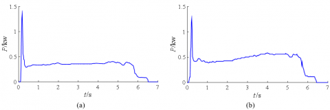
Based on the historical data of the power curve of the S700K turnout from the Signal Centralized Monitoring Center of Lanzhou Railway Corporation and taking 40ms as the sampling period, this paper summarizes the power curves under four typical running states of healthy, sub-healthy, fault, and severe fault, as shown in Figure 2. The corresponding classification analysis is shown in Table 1.
Figure 2. Power curve of typical running state of S700K turnout
Table 1. Classification and analysis of power curve of S700K turnout under typical running state
|
Code |
Running state |
Curve type |
Power curve characteristics |
|
(a) |
Healthy |
Normal power curve |
Unlock peak value, smooth transition, lock "small steps" |
|
(b) |
Sub-healthy 1 |
Represents loop current is too large |
The "small step" in the locking phase is slightly larger than the normal curve |
|
(c) |
Sub-healthy 2 |
The installation of switch rods and other devices is not standard or loose |
The curve fluctuates during the conversion phase, but the conversion action can be completed |
|
(d) |
Fault 1 |
Rectifier stack open circuit |
"Small steps" disappear in the locking phase |
|
(e) |
Fault 2 |
Diode short circuit |
The "small steps" in the locking phase are about twice as high as normal |
|
(f) |
Severe fault |
Switch split |
The conversion time is too long and the motor idles |
The power curve characteristics of turnout can be roughly divided into three stages: start unlocking, conversion and locking. In the unlocking stage, the action power curve in the healthy state has a peak value due to the hard start of the motor, and the conversion stage is relatively stable. In the locking stage, there are "small steps" due to the circuit composed of two-phase currents B, C and rectifier stack. When the S700K turnout is in the sub-health state between health and fault, the power curve of changes slightly, such as the vibration in the transition stage and the circuit current is too large. When the S700K turnout is in fault mode, the representation circuit of the S700K turnout is abnormal due to rectifier stack and diode failure. In the severe failure mode, the turnout is crowded due to the presence of foreign bodies, resulting in a longer conversion time.
4.2 Frequency domain analysis of power curve
In the diagnosis of the full cycle running state of the S700K turnout, the power curve is classified into four typical running states: health, sub-health, fault, and severe fault. Under different running states, some power curves show obvious characteristics, such as long transition time under serious faults, while some action power curves only show weak characteristics, such as the curve characteristic of excessive loop current and vibration in the transition phase is low. To reflect the weak characteristics of the power curve under different running states, this paper uses the VMD to extract the detailed components of the power curve.
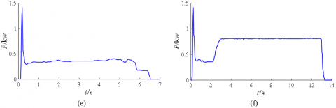
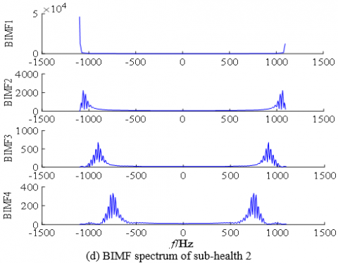
According to the method of observation center frequency in Reference [19], when the decomposition level K = 4, the penalty factor α = 1000, the difference of center frequency is large and the signal recognition is high. Taking the running state of the S700K turnout in sub-health 1 and sub-health 2 as an example, the four BIMF and corresponding spectrum after VMD are shown in Figure 3.
From the VMD results and spectrum analysis, it is apparent seen that the spectrum distribution centers of BIMF in the same running state are different. As shown in Figure 3(b), the center frequency of the envelope spectrum of BIMF1 is higher than 1,000 and the center frequencies of BIMF2-BIMF4 decrease successively. The spectrum distribution centers of the same BIMF in the different running states are similar, and the differences of spectrum amplitudes are small. To characterize the effective features of BIMF of different power curves, MPE is used to calculate the modal components, and the feature sets are further analyzed.
Figure 3. BIMF and corresponding spectrum of S700K turnout
4.3 Entropy calculation and analysis
To quantitatively describe the effective characteristics of the power curve, MPE is used to illustrate the signal complexity of the BIMF component. Supposing that the one-dimensional signal sequence is x, and the coarse-grained signal sequence is y, and the time scale is τ, the MPE is shown in Eq. (24).
$\operatorname{MPE}(\boldsymbol{x}, \tau, m, \delta)=\operatorname{PE}\left(\boldsymbol{y}_{j}^{\tau}, m, \delta\right)$ (24)
where PE is the permutation entropy, MPE is the multi-scale permutation entropy, and $m$ and $\delta$ represent embedding dimension and delay parameters respectively.
In practice, the sampling of the microcomputer monitoring center is 40 ms, so when the S700K turnout is running normally, the sampling point N is 165. In Ref. [20], N≥5m!, therefore, m is taken as 4, τ is usually less than 2. Taking the S700K turnout in a healthy state as an example, and then delaying parameters δ is 5, the original feature set R5x5 is established by the power curve and BIMF in healthy state:
$\boldsymbol{R}=\left[\begin{array}{lllll}0.840 & 0.830 & 0.888 & 0.922 & 0.801 \\ 0.448 & 0.490 & 0.523 & 0.559 & 0.609 \\ 0.603 & 0.740 & 0.835 & 0.907 & 0.940 \\ 0.765 & 0.928 & 0.986 & 0.964 & 0.887 \\ 0.998 & 0.995 & 0.983 & 0.993 & 0.998\end{array}\right]$
The correlation of the above feature sets is different and there is signal redundancy, which cannot be used as input signals for fuzzy clustering analysis. To simplify the signal characteristics, the KPCA is carried out on the feature set R, and the parameters with the cumulative contribution rate of more than 95% of the feature values are selected as the new eigenvector $\overline{\boldsymbol{R}}$. Taking the feature set of the S700K turnout in a health state as an example, after KPCA analysis, the new eigenvector $\overline{\boldsymbol{R}}$ is:
$\overline{\boldsymbol{R}}=\left[\begin{array}{llll}4.103 & 0.062 & 0.062 & 0\end{array}\right]$
The feature vector $\overline{\boldsymbol{R}}$ can satisfy the requirement of no loss of signal features and eliminate information redundancy, which greatly reduces the calculation of state diagnosis.
4.4 Running state diagnosis of S700K turnout
4.4.1 Running state diagnosis model of turnout
Through the frequency-domain analysis of the power curve of the S700K turnout, based on the power curve (a) to (f) in the typical running state in Figure 2, the eigenvector after KPCA analysis is shown in Table 2.
Table 2. Sample eigenvector in different states of turnout
|
Code |
Eigenvector |
|||
|
(a) |
4.103 |
0.062 |
0.062 |
0.009 |
|
(b) |
3.830 |
0.099 |
0.094 |
0.094 |
|
(c) |
3.945 |
0.043 |
0.014 |
0.014 |
|
(d) |
3.972 |
0.101 |
0.041 |
0.005 |
|
(e) |
4.124 |
0.088 |
0.064 |
0.064 |
|
(f) |
3.920 |
0.070 |
0.014 |
0.014 |
Each group of power curves of the S700K turnout under different typical running states is taken as the sample object, and curves (a) to (f) are defined to indicate their eigenvectors by f0 ~ f5. The fuzzy clustering algorithm is used to carry out clustering analysis, which will establish the running state diagnosis model of the S700K turnout.
Step 1: Establish fuzzy matrix X.
$X=\left[f_{0} ; f_{1} ; f_{2} ; f_{3} ; f_{4} ; f_{5}\right]$ (25)
Step 2: Fuzzy matrix normalization X′′.
The fuzzy standard matrix X′′ is obtained by using Eqns. (13) and (14):
$\boldsymbol{X}^{\prime \prime}=\left[\begin{array}{cccc}0.928 & 0.327 & 0.600 & 0.044 \\ 0 & 0.965 & 1 & 1 \\ 0.391 & 0 & 0 & 0.101 \\ 1 & 0.775 & 0.625 & 0.662 \\ 0.306 & 0.465 & 0 & 0.101\end{array}\right]$
Step 3: Establish fuzzy similarity matrix R.
As shown in Eq. (15), the fuzzy similarity matrix R is established using the exponential similarity coefficient method:
$\boldsymbol{R}=\left[\begin{array}{lrrrrr}1 & 0.433 & 0.677 & 0.685 & 0.716 & 0.675 \\ 0.433 & 1 & 0.370 & 0.521 & 0.579 & 0.456 \\ 0.677 & 0.370 & 1 & 0.606 & 0.520 & 0.824 \\ 0.685 & 0.521 & 0.606 & 1 & 0.660 & 0.754 \\ 0.716 & 0.579 & 0.520 & 0.660 & 1 & 0.580 \\ 0.675 & 0.456 & 0.824 & 0.754 & 0.580 & 1\end{array}\right]$
Step 4: Constructing fuzzy equivalence matrix R*.
As shown in Eq. (16), the fuzzy equivalent matrix R* is constructed using the transfer packet algorithm:
$\boldsymbol{R}^{*}=\left[\begin{array}{llllll}1 & 0.579 & 0.685 & 0.685 & 0.716 & 0.685 \\ 0.579 & 1 & 0.579 & 0.579 & 0.579 & 0.579 \\ 0.685 & 0.579 & 1 & 0.754 & 0.685 & 0.824 \\ 0.685 & 0.579 & 0.754 & 1 & 0.685 & 0.754 \\ 0.716 & 0.579 & 0.685 & 0.685 & 1 & 0.685 \\ 0.685 & 0.579 & 0.824 & 0.754 & 0.685 & 1\end{array}\right]$
Step 5: Form cluster diagram.
Eq. (17) is used to establish the corresponding equivalent Boolean matrix Rλ. When λ changes from 1 to 0, the same columns of the matrix Rλ are grouped into one category, and a dynamic cluster diagram is formed, thereby completing the establishment of the S700K turnout running state diagnosis model.
4.4.2 Diagnostic results and state analysis of the curves to be tested
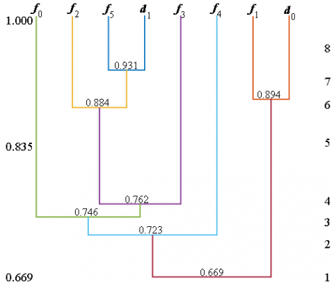
To verify the effectiveness of the diagnostic model for the running state of the S700K turnout, based on the historical monitoring data of S700K turnout from the signal centralized monitoring center of Lanzhou Railway Corporation, power curves are randomly selected under sub-health 1 and severe fault conditions. Each curve data is regarded as the curve to be tested, and its label is defined as d0 ~ d1. After the frequency-domain analysis and feature analysis, the eigenvectors of the power curves to be tested are shown in Table 3. Combined with the diagnosis model in the previous section, the eigenvectors of the power curves to be tested are analyzed by fuzzy clustering, and the dynamic clustering diagram is shown in Figure 4.
Table 3. Eigenvector of the power curve to be tested
|
Code |
Eigenvector |
|||
|
d0 |
4.103 |
0.062 |
0.062 |
0.009 |
|
d1 |
3.920 |
0.070 |
0.014 |
0.014 |
From the dynamic clustering diagram of the power curve to be tested, when the λ on the left changes from 1 to 0, the number of categories on the right decreases and finally falls into one category. When λ changes to 0.931, f5 and d1 are classified into one category, and the curve d1 to be tested and the sample f5 belongs to the same state, so d1 is diagnosed as sub-health 1. Similarly, when λ changes to 0.849, f1 and d0 are classified into one category, d0 is diagnosed as a serious fault state, which is consistent with the field detection results.
Due to the low failure rate of S700K turnout and the difficulty in sample collection, this paper uses MATLAB software to carry out fuzzy clustering simulation analysis of the curves under different running states. The state diagnosis of S700K turnout can be realized without a large amount of data for training. To verify the effectiveness of the algorithm, 10 groups of power curves of S700K turnout under different running states are taken as the test set. A total of 60 sets are input into the state diagnosis model one by one, the results show that the F-measure is 93.23%, which verifies the effectiveness of the proposed algorithm.
Figure 4. Dynamic clustering diagram of the power curve to be tested
Aiming at the consistency between the running state and the power curve of the S700K turnout, this paper proposes to use VMD for frequency domain analysis, combined with KPCA to extract the characteristics of the power curve. The fuzzy clustering analysis algorithm is used to realize the diagnosis algorithm of S700K turnout's full cycle running state, and the following conclusions are drawn:
1) The decomposition method of VMD has the characteristics of self-adaptation, and it can be used to analyze the power curve in frequency domain, which is beneficial to extract the detail components of S700K turnout.
2) Multi-scale permutation entropy is an index to measure signal complexity, and it is sensitive to signal mutations. It can be used to characterize the micro characteristics of power curves and decomposition components. KPCA eliminates the redundancy of feature information and improves the recognition rate and efficiency of running state diagnosis.
3) The different running states of S700K turnout are used to form a dynamic clustering diagram. When the λ takes a specific value, the running state diagnosis of S700K turnout is realized. The experimental results show that the algorithm has the characteristics of small sample analysis, and does not need to be trained in advance. It can realize the diagnosis of the state of the S700K turnout, and provide a new guarantee for its equipment maintenance and repair.
This work was supported in part by the National Natural Science Foundation of China (Grant numbers: 61661027).
[1] Gao, L.M., Xu, Q.Y., Li, F. (2020). Research on degradation state of turnout equipment based on SOM-BP hybrid neural network. China Railway Science, 41(03): 50-58. https://doi.org/10.18280/ijht.350401
[2] Ji, W., Chen, C., Xie, G., Zhu, L., Hei, X. (2021). An intelligent fault diagnosis method based on curve segmentation and SVM for rail transit turnout. Journal of Intelligent and Fuzzy Systems, 1: 1-11. https://doi.org/10.3233/JIFS-189688
[3] Cong, C., Tianhua, X., Guang, W., Bo, L. (2021). Railway turnout system RUL prediction based on feature fusion and genetic programming. Measurement, 151: 107162. https://doi.org/10.1016/j.measurement.2019.107162
[4] Eker, O.K., Camci, F., Guclu, A., Yilboga, H., Baskan, S. (2011). A simple state-based prognostic model for railway turnout systems. IEEE Transactions on Industrial Electronics, 58(5): 1718-1726. http://dx.doi.org/10.1109/TIE.2010.2051399
[5] Yang, J.H., Yu, Y.J., Chen, G.W. (2020). Research on turnout fault diagnosis algorithms based on CNN-GRU model. Journal of the China Railway Society, 42(07): 102-109. http://dx.doi.org/10.3969/j.issn.1001-8360.2020.07.013
[6] Wei, W.J., Liu, X.F. (2019). Fault diagnosis of S700K switch based on EEMD multi-scale sample entropy. Journal of Central South University (Science and Technology), 50(11): 2763-2772. http://dx.doi.org/10.11817/j.issn.1672-7207.2019.11.015
[7] Zhong, Z., Chen, J., Tang, T., Xu, T., Wang, F. (2018). SVDD-based research on railway-turnout fault Detection and health assessment. Journal of Southwest Jiaotong University, 53(4): 842-849. http://dx.doi.org/10.3969/j.issn.0258-2724.2018.04.024
[8] Zhou, X.X., Wang, X.M., Yang, Y., Guo, J., Wang, P. (2014). De-noising of high-speed turnout vibration signal based on wavelet threshold. Journal of Vibration and Shock, 33(23): 200-206. http://dx.doi.org/10.13465/j.cnki.jvs.2014.23.036
[9] Zhang, K., Du, K., Ju, Y.F. (2014). Algorithm of railway turnout fault detection based on PNN neural network. 2014 Seventh International Symposium on Computational Intelligence and Design, pp. 544-547. http://dx.doi.org/10.1109/iscid.2014.140
[10] Zhao, L.H., Lu, Q. (2014). Method of turnout fault diagnosis based on grey correlation analysis. Journal of the China Railway Society, 36(2): 69-74. http://dx.doi.org/10.3969/j.issn.1001-8360.2014.02.011
[11] Gong, T.K., Yuan, X.H., Yuan, Y.B., Lei, X.H., Wang, X. (2018). Application of tentative variational mode decomposition in fault feature detection of rolling element bearing. Measurement, 135: 481-492. http://dx.doi.org/10.1016/j.measurement.2018.11.083
[12] Li, C., Cerrada, M., Cabrera, D., Sanchez, R., Pacheco, F., Ulutagay, G., Valente, O.J. (2018). A comparison of fuzzy clustering algorithms for bearing fault diagnosis. Journal of Intelligent & Fuzzy Systems, 34(6): 3565-3580. http://dx.doi.org/10.3233/JIFS-169534
[13] Tang, S.P., Peng, G., Zhong Z.X. (2016) An improved fuzzy C-means clustering algorithm for transformer fault. 2016 China International Conference on Electricity Distribution (CICED), pp. 1-5. http://dx.doi.org/10.1109/CICED.2016.7576369
[14] Rabcan, J., Levashenko, V., Zaitseva, E., Kvassay, M., Subbotin, M. (2019). Non-destructive diagnostic of aircraft engine blades by Fuzzy Decision Tree. Engineering Structures, 197: 109396. http://dx.doi.org/10.1016/j.engstruct.2019.109396
[15] Dragomiretskiy, K., Zosso, D. (2014). Variational mode decomposition. IEEE Transactions on Signal Processing, 62(3): 531-544. http://dx.doi.org/10.1109/TSP.2013.2288675
[16] Jiang, X.X., Wang, J., Shi, J.J., Shen, C.Q., Huang, W.G., Zhu, Z.K. (2019). A coarse-to-fine decomposing strategy of VMD for extraction of weak repetitive transients in fault diagnosis of rotating machines. Mechanical Systems and Signal Processing, 116: 668-692. http://dx.doi.org/10.1016/j.ymssp.2018.07.014
[17] Zhang, X., Miao, Q., Zhang, H., Wang, L. (2018). A parameter-adaptive VMD method based on grasshopper optimization algorithm to analyze vibration signals from rotating machinery. Mechanical Systems and Signal Processing, 108: 58-72. http://dx.doi.org/10.1016/j.ymssp.2017.11.029
[18] Sun, H., Guo, Y.Q., Zhao, W.L. (2020). Fault detection for aircraft turbofan engine using a modified moving window KPCA. IEEE Access, 8: 166541-166552. http://dx.doi.org/10.1109/ACCESS.2020.3022771
[19] Liu, C.L., Wu, Y., Zhen, C. (2015). Rolling bearing fault diagnosis based on variational mode decomposition and fuzzy C means clustering. Proceedings of the Chinese Society of Electrical Engineering, 35(13): 3358-3365. http://doi.org/10.13334/j.0258-8013.pcsee.2015.13.020
[20] Matilla-García, M. (2007). A non-parametric test for independence based on symbolic dynamics. Journal of Economic Dynamics and Control, 31(12): 3889-3903. http://dx.doi.org/10.1016/j.jedc.2007.01.018