Lucien Duclos Ndoumbe | Samuel Eke | Charles Hubert Kom* | Aurélien Tamtsia Yeremou | Arnaud Nanfak | Gildas Martial Ngaleu
© 2021 IIETA. This article is published by IIETA and is licensed under the CC BY 4.0 license (http://creativecommons.org/licenses/by/4.0/).
OPEN ACCESS
This paper is in the field of electric power quality monitoring and presents a new approach for the identification, classification and characterization of the nine voltage dips and swells in electricity networks. The proposed method is based on the study in the complex plane of the signatures of the different voltage dips and swells. In the study of these signatures, the elements taken into account are the root mean square (RMS) values of the phases, the existence or not of an additional phase shift of the voltages and their rotation sense. The informations obtained are synthesized in three variables, and used to the implementation of the method. The results found by the computer simulations carried out by the MATLAB/Simulink software show that the proposed approach uses few parameters, is easy to implement and understand, and makes it possible to efficiently detect, classify and characterize the nine voltage dips and swells.
power quality, voltage dips, voltage swells, signatures
Power Quality problems are defined as any power problems manifested in voltage, current, or frequency deviation that results in failures or malfunctions of customers equipments [1]. Voltage dips and swells are the two recurrent disturbances affecting voltage magnitude. Voltage dips, also known as voltage sags are one of the most serious problems of electric power quality and represent a major handicap for the industrial and domestic consumers [2]. The voltage dip is a sudden drop in voltage at a point of the power system to a value between 90% and 1% (IEC 61000-2-1) or between 90% and 1% (IEEE 1159) of a reference voltage. This affects one or more phases, followed by a voltage recovery after a short period of time between the fundamental half-period of the system (10 ms to 50 Hz) and one minute [3]. Voltage dips are mainly caused by short circuits, earth faults in the power grid or connected installations, and high current demands due to the starting of large induction motors, arcs or transformer saturation [4, 5]. They affect the operation of control devices, such as unintentional opening of contactors and relays, cause switching faults in inverters, malfunctions in analogue or digital electronic systems, and errors in the execution of computer calculations [6]. On the other hand, the rise in voltage that occurs when a voltage dip disappears causes an overcurrent in rotating machines, leading to the creation of heat sources and short duration electrodynamics forces that can have long term effects such as ageing [7]. As opposed to voltage dip, the voltage swell is a rise in voltage at a point of the power system to a value between 110% and 180% of the normal voltage for duration from half a cycle to several seconds. It occurs when heavy load is turned off, when loss of generation, badly regulated transformer, faulty conditions at various points in the AC distribution system, under loading of a phase while other two phases in a 3-phase system are overloaded Johnson and Hassan [8] or by intermittent renewable energies connected to the grid [9, 10].
During the last decades, equipment’s used in the industrial sector have become more sensitive to voltage dips and swells due to recent advances and the increasing use of power electronics devices [11]. Due to all this, the implementation of methods for the detection, classification and characterization of voltage dips has become an essential condition for monitoring the quality of electrical power, which represents the preliminary step in the search of solutions. The characterization of voltage dips allows extracting informations about the causes of dip, location of the fault in the grid and states of the grid when the fault occurs.
In order to detect, analyze and determine the type of voltage dip, several methods are proposed in the literature. Among these methods, we have the 6-voltages method which compares the RMS values of the 6 simple and compound voltages [12]. The type of voltage dip is determined from the lowest RMS value. This method does not provide any information on the affected phases and does not allow the classification of different types of voltage dips and swells. The symmetrical component method [13, 14] which determines only three types of voltage dips by studying the complex plane of forward and reverse voltages. Eke and Imano [15] proposed an exhaustive classification algorithm of the nine types of voltage dips and swells based on a combination of the 6-voltages and symmetrical component methods. Another classification approach, the space vector method, was presented by Ignatova et al. [16]. This method is based on the transformation of the space vector, which describes the three-phase voltage system by a complex variable: the space vector. For Alam et al. [17], a new approach based on polarization ellipse in 3-D coordinates is proposed. This approach exploits signatures and parameters of three-phase voltage signals. Five parameters extracted of ellipse including azimuthal angle, elevation, tilt, semi-minor axis and semi-major axis are used to classify and characterize. Ma et al. [18] proposed a new algorithm based on the shapes of Type C and Type D for calculating the voltage dip type. Some technics are using Kalman Filtering Models such as Extented Kalman Filtering Algorithms for overcoming the limitations of Linear Kalman Filters [19], which offers accuracy in the optimal estimation of the magnitude, duration of voltage dips and phase angle jump are proposed in refs. [20, 21]. Fourier Transform Methods are studied and produce accurate results which generate significant delay in the response of the system to voltage sags by extraction of informations from a signal in the frequency domain [22, 23]. Other Methods on Numerical Matrix Sag Detection are also developed by analysing different harmonics present in the supply voltages [24]. Another approach based on analysis of the envelope of the voltage network is used to detect the voltage dip determined by locating the Signal Local Maximums is presented by Boujoudi et al. [25]. These local maximums are calculated by using an algorithm founded on the detection of the sign changing of two consecutive samples of the signal difference. With the development of artificial intelligence tools, several intelligent classifiers of voltage dips are proposed in the literature. For instance, many Learning Machine Algorithms such as K-Means-Clustering, Logistic Regression Algorithms and others are developed for characterization of recorded voltage dips and real-time measured voltage data [26, 27]. A dip type identification algorithm based on K-means-Singular Value decomposition and Least Squares Support Vector Machine is presented by Axelberg et al. [28]. According to Sha et al. [29], a support vector machine (SVM) classifier using five time-frequency domain features extracted from the RMS waveform of voltage dips is proposed. The features are used as the training data of the SVM to realize the identification of the voltage dip type. In Adegbite and Okelola [1], a naive Bayes classifier is proposed for the classification of voltage dips and swells.
In this paper, a new approach for the classification and characterization of voltage dips is proposed. It is based on the signatures of the different voltage dips. This method allows an exhaustive classification and a complete characterization of three-phase voltage dips. All computer simulations were performed in MATLAB/Simulink software.
After the Introduction section, the remaining part of this paper is organized as follows: Section II presents the nine types of voltage dips and swells and their complex representations. The principle of proposed method is described in Section III. Section IV presents the platform and simulation results. A conclusion is given in section V.
Voltage dips and swells are characterized by their depth amplitude and duration. In addition to duration and amplitude, three-phase voltage dips are characterized by the phase shift between the phase voltages [2]. Three-phase voltage dips and swells are often analysed in the complex plane, where the three voltages are represented as vectors characterised by their amplitude and phase, also called phasors. The relationship between the phasors in the complex plane is called the signature [16]. The signature vectors associated at types of voltage dips and swells are presented in Table 1.
Table 1. Voltage dips and swells types and signature vectors
|
Dips Types |
Single phase dip |
Two-phase dips |
Three-phase dips |
|
|
Without phases shift |
Without swell |
|||
|
(b) Type B |
(e) Type E |
(a) Type A |
||
|
With phases shift |
|
|||
|
(d) Type D |
(c) Type C |
|||
|
(f) Type F |
(g) Type G |
|||
|
With swell |
||||
|
(h) Type H |
(i) Type I |
|||
Dip and swell signatures depend on several parameters such as voltage dip cause, voltage dip location and system grounding. The ABC voltage dip classification is based on the fault type which leads to the dip. According to this classification, all voltage dips are classified into seven dip types namely A, B, C, D, E, F and G dip types [30] and two types of voltage swells namely H and I [16].
The parameters that characterize the signature vector are:
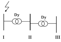
The signature of the voltage dips can be modified by the transformers located within the network. The Figure 1 and Table 2 below present the different dips that propagate downstream of the network, through the most commonly used Dy transformers.
Figure 1. Transformations of voltage dip types [31]
Table 2. Propagation of voltage dips [31]
|
Voltage level |
Types of voltage dips |
||||
|
I |
A |
B |
C |
E |
- |
|
II |
A |
C |
D |
F |
H, I |
|
III |
A |
D |
C |
G |
- |
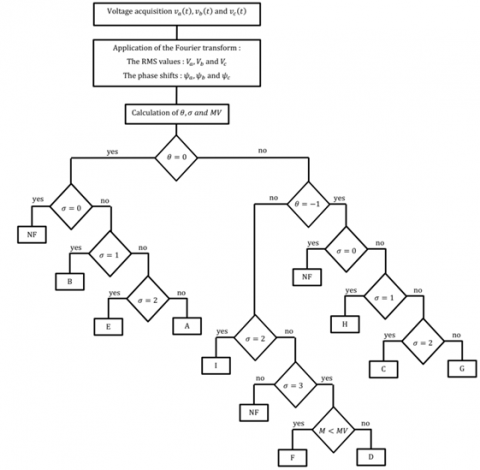
In this paper, it is proposed a new algorithm of classification for voltage dips and swells. This new method consists to detect, to classify and to characterize the nine types of voltage dips and swells, in order to implement a process and monitor a power supply quality. This new approach exploits the signature vectors of the different voltage dips and swells. In the study of these signatures, we take into account the amplitude of the RMS values, the existence or not of additional phase shift and their rotation sense for each phase. From the study of the different signatures, the detection and classification of the different voltage dips can be summarized by the study of the three parameters θ, σ and MV defined as follow.
The parameter θ, informs us about the existence or not of additional phase shifts and its rotation sense. This parameter is calculated from the phase shifts between the different phases. The increase or decrease of these phase shifts in relation to the normalised value of $\frac{2 \pi}{3}$ is an indication of the existence of an additional phase shift, of the phases concerned and of its rotation sense. A study of the signatures of the different voltage dips and swells allowed us to establish the relationship between the values of θ and the different types of voltage dips and swells:
The parameter σ informs us about the presence or absence of voltage reduction on the phases. The values of σ are defined on the basis of the RMS values Va, Vb and Vc of the three phases. A study of the signatures of the different voltage dips and swells has enabled us to establish the relationship between the values of σ and the different types of voltage dips and swells:
Figure 2. Algorithm of proposed method for voltage dips classification
Table 3. Propagation of voltage dips [4]
|
Fault |
Parameters |
||
|
m |
a |
d |
|
|
A |
/ |
/ |
$1-\min \left( {{V}_{a}},{{V}_{b}},{{V}_{c}} \right)$ |
|
B |
/ |
/ |
$1-\min \left( {{V}_{a}},{{V}_{b}},{{V}_{c}} \right)$ |
|
C |
$\min \left( {{V}_{a}},{{V}_{b}},{{V}_{c}} \right)$ |
${{\sin }^{-1}}\left( \frac{1}{2m} \right)-30{}^\circ $ |
$1-m\cos \left( \alpha \right)$ |
|
D |
$\max \left( {{V}_{a}},{{V}_{b}},{{V}_{c}} \right)$ |
${{\tan }^{-1}}\left( \frac{d\sqrt{3}}{4-d} \right)$ |
$1-\min \left( {{V}_{a}},{{V}_{b}},{{V}_{c}} \right)$ |
|
E |
/ |
/ |
$1-\min \left( {{V}_{a}},{{V}_{b}},{{V}_{c}} \right)$ |
|
F |
$\max \left( {{V}_{a}},{{V}_{b}},{{V}_{c}} \right)$ |
${{\tan }^{-1}}\left( \frac{d}{\sqrt{3}\left( 2-d \right)} \right)$ |
$1-\min \left( {{V}_{a}},{{V}_{b}},{{V}_{c}} \right)$ |
|
G |
$\min \left( {{V}_{a}},{{V}_{b}},{{V}_{c}} \right)$ |
${{\cos }^{-1}}\left( \frac{1-d}{m} \right)$ |
$\frac{5\left( 1-\max \left( {{V}_{a}},{{V}_{b}},{{V}_{c}} \right) \right)}{2}$ |
|
H |
$\max \left( {{V}_{a}},{{V}_{b}},{{V}_{c}} \right)$ |
${{\tan }^{-1}}\left( \frac{d\sqrt{3}}{2+d} \right)$ |
$1-\min \left( {{V}_{a}},{{V}_{b}},{{V}_{c}} \right)$ |
|
I |
$\min \left( {{V}_{a}},{{V}_{b}},{{V}_{c}} \right)$ |
${{\tan }^{-1}}\left( \frac{d\sqrt{3}}{1-d} \right)$ |
$\frac{\left( \max \left( {{V}_{a}},{{V}_{b}},{{V}_{c}} \right)-1 \right)}{2}$ |
The variable MV is used to separate voltage dips of type D and F, having almost similar signatures. The idea for this parameter comes from the work of Eke and al., but there is a difference in the expression of the MV parameter against the one defined in [15]. Indeed, we use:
$M V=\frac{\sqrt{3}}{2} V_{R M S}$ (1)
Instead of:
$M V=\frac{2}{3} V_{R M S}$ (2)
VRMS is the RMS value of the reference voltage.with,
We have then:
with Va, Vb and Vc and the RMS values of phases a, b and c respectively.
All the relationships established between the parameters and the different voltage dips are summarized in the algorithm in Figure 2.
The characterization of the voltage dip after detection and classification is carried out graphically, by indication of phases that have undergone a voltage drop and an additional phase shift. In addition to this information, the depth, duration and angle of the additional phase shift are given. All these informations can contribute to the identification of the cause of the fault, and by dip spectrum analysis, at the location of the fault. Table 3 summarizes the expressions of the characteristic parameters of the different voltage dips and swells.
A three-phase 230/380 V electrical network with a frequency of 50 Hz has been considered for the simulation. Then, in Simulink, we have introduced single-, two- and three-phase faults of type A, B and E respectively. To generate the other voltage dips and swells, Dy transformers have been used in order to modify the signature of voltage dips according to Table 4. The voltage dips and swells analyser receive the single voltages as input and returns the dip type or swell type and the voltage fault characterization elements as output. The MATLAB/Simulink platform is shown in Figure 3.
Simulation results are summarized in three categories of variables:
Table 4. Classification legend
|
ρ |
Voltage dip |
|
0 |
ND |
|
1 |
A |
|
2 |
B |
|
3 |
C |
|
4 |
D |
|
5 |
E |
|
6 |
F |
|
7 |
G |
|
8 |
H |
|
9 |
I |
Figure 3. Simulink model of simulation
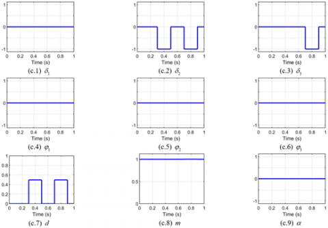
The characterization variables $d, m, \alpha, \delta_{i ; i=1,2,3}$ (which informs us on the phases having undergone a voltage drop or overvoltage) and $\varphi_{i ; i=1,2,3}$ (which informs us on the phases having undergone an additional phase shift). $\delta_{i}=1$ in case of overvoltage, $-1$ in case of voltage drop and 0 in the opposite case. $\varphi_{i}=1$ if the phase has undergone an additional phase shift and 0 if not.
The results presented in this section are the result of a series of measurements made from simulations on our power grid. Indeed, we carry out the marking of the nine voltage dips and swells known to date from the detection, classification and characterisation blocks carried out from the variables obtained from studying their different signatures. It should be noted that MV is a relevant parameter only for voltage dips of type D and type F only; similarly, the variable m is not relevant for voltage dips without additional phase shift namely A, B and E.
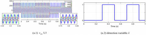
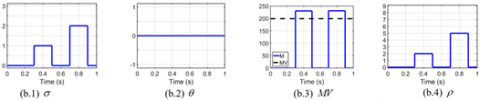
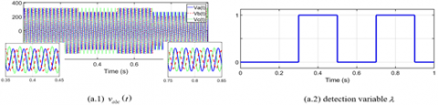
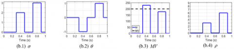
Figure 4 presents the results of a A-type voltage dip affecting all phases and occurring between 0.3s and 0.5s as illustrated in (a.1), as well as the corresponding detection, classification and characterisation variables. We observe that the detection variable λ in (a.2) is equal to 1 between 0.3s and 0.5s. In (b.1) and (b.2), the method variables indicate that all three phases are affected by the fault (σ=3) and there is no additional phase shift (θ=0). From these values, we obtain in (b.4) the value of the classification variable ρ=1 which indicates that it is a A-type voltage dip. Concerning the characterization variables, the amplitude variables in (c.1) δ1=-1, (c.2) δ2=-1 and (c.3) δ3=-1 indicate voltage drops of more than 10% of the reference value of the three phases. Similarly, the additional phase shift variables in (c.4) φ1=0, (c.5) φ2=0 and (c.6) φ3=0 indicate that none of the phases are subject to additional phase shift. This is verified by the value of the additional phase shift α=0 in (c.9).
From this, it can be deduced that the fault is a three-phase voltage dip with a dip depth of 50% (c.7) without additional phase shift.
(a) Three-phase voltage and detection variable
(b) Parameters and classification variables
(c) Characterization variables
Figure 4. A-type voltage dip
(a) Three-phase voltage and detection variable
(b) Parameters and classification variables
(c) Characterization variables
Figure 5. B and E-type voltage dips
(a) Three-phase voltage and detection variable
(b) Parameters and classification variables
(c) Characterization variables
Figure 6. C and F-type voltage dips
Figure 5 presents the results of B-type (affecting only one phase) and E-type (affecting two phases) voltage dips occurring respectively between 0.3s and 0.5s and between 0.7s and 0.9s as illustrated in (a.1) as well as the corresponding detection, classification and characterization variables. We observe that the detection variable λ in (a.2) is equal to 1 twice, the first time between 0.3s and 0.5s and the second time between 0.7s and 0.9s.
Between 0.3s and 0.5s, the variables of the method in (b.1) and (b.2), indicate that one of the three phases is affected by the fault (σ=1) and there is no additional phase shift (θ=0). From these values, we obtain in (b.4) the value of the classification variable ρ=2 which indicates that it is a B-type voltage dip. Concerning the characterization variables, the amplitude variables in (c.1) δ1=0, (c.2) δ2=-1 and (c.3) δ3=0 indicate voltage drops of more than 10% of the reference value on phase b. Between 0.7s and 0.9s, the variables of the method in (b.1) and (b.2), indicate that two of the three phases are affected by the fault (σ=2) and there is no additional phase shift (θ=0). From these values, we obtain in (b.4) the value of the classification variable ρ=5 which indicates that it is a E-type voltage dip. Concerning the characterization variables, the amplitude variables in (c.1) δ1=0, (c.2) δ2=-1 and (c.3) δ3=-1 indicate voltage drops of more than 10% of the reference value on phase b and phase c. The additional phase shift variables in (c.4) φ1=0, (c.5) φ2=0 and (c.6) φ3=0 indicate that none of the phases are subject to additional phase shift in both cases. We deduce that between 0.3s and 0.5s the fault is a single-phase voltage dip with a dip depth of 50% (c.7) without additional phase shift and between 0.7s and 0.9s the fault is a two-phase voltage dip with a dip depth of 50% (c.7) without additional phase shift.
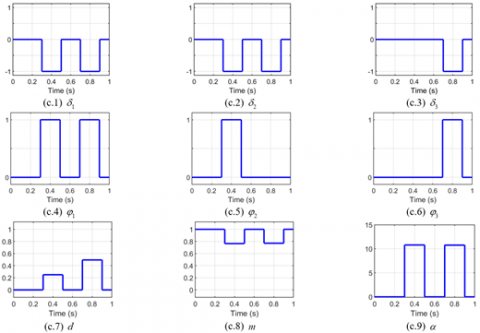
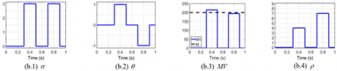
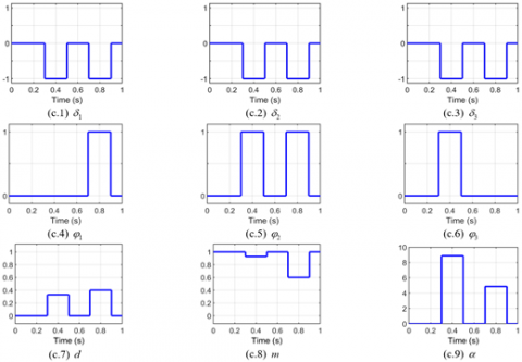
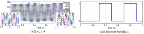
Figure 6 presents the results of C-type (affecting two phases) and F-type (affecting three phases) voltage dips occurring respectively between 0.3s and 0.5s and between 0.7s and 0.9s as illustrated in (a.1) as well as the corresponding detection, classification and characterization. We observe that the detection variable λ in (a.2) is equal to 1 twice, the first time between 0.3s and 0.5s and the second time between 0.7s and 0.9s. Between 0.3s and 0.5s, the variables of the method in (b.1) and (b.2), indicate that two of the three phases are affected by the fault (σ=2) and there is an additional counter-clockwise phase shift (θ=-1)From these values, we obtain in (b.4) the value of the classification variable ρ=3 which indicates that it is a C-type voltage dip. Concerning the characterization variables, the amplitude variables in (c.1) δ1=-1, (c.2) δ2=-1 and (c.3) δ3=0 indicate voltage drops of more than 10% of the reference value on phases a and b. The additional phase shift variables in (c.4) φ1=1, (c.5) φ2=1 and (c.6) φ3=0 indicate that these are the phases a and b that have an additional phase shift. We deduce that between 0.3s and 0.5s the fault is a two-phase voltage dip with a dip depth of 22% (c.7) with additional phase shift of 11° (c.9).
Between 0.7s and 0.9s, the variables of the method in (b.1), (b.2) and (b.3), indicate that all three phases are affected by the fault (σ=3), there is an additional clockwise phase shift (θ=1) and the maximum RMS value M is lower than the value of the parameter MV. From these values, we obtain in (b.4) the value of the classification variable ρ=6 which indicates that it is a F-type voltage dip. Concerning the characterization variables, the amplitude variables in (c.1) δ1=-1, (c.2) δ2=-1 and (c.3) δ3=-1 indicate voltage drops of more than 10% of the reference value of the three phases. The additional phase shift variables in (c.4) φ1=1, (c.5) φ2=0 and (c.6) φ3=1 indicate that these are the phases a and c that have an additional phase shift. We deduce that between 0.7s and 0.9s the fault is a three-phase voltage dip with a dip depth of 50% (c.7) with additional phase shift of 11° (c.9).
Figure 7 presents the results of D-type and G-type voltage dips (affecting three phases) occurring respectively between 0.3s and 0.5s and between 0.7s and 0.9s as illustrated in (a.1) as well as the corresponding detection, classification and characterisation. We observe that the detection variable λ in (a.2) is equal to 1 twice, the first time between 0.3s and 0.5s and the second time between 0.7s and 0.9s.
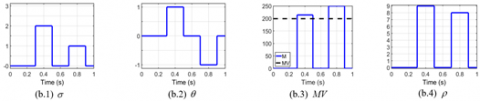
Between 0.3s and 0.5s, the variables of the method in (b.1), (b.2) and (b.3), indicate that all three phases are affected by the fault (σ=3), there is an additional clockwise phase shift (θ=1) and the maximum RMS value M is upper than the value of the parameter MV. From these values, we obtain in (b.4) the value of the classification variable ρ=4 which indicates that it is a D-type voltage dip. Concerning the characterization variables, the amplitude variables in (c.1) δ1=-1, (c.2) δ2=-1 and (c.3) δ3=-1 indicate voltage drops of more than 10% of the reference value of the three phases. The additional phase shift variables in (c.4) φ1=0, (c.5) φ2=1 and (c.6) φ3=1 indicate that these are the phases b and c that have an additional phase shift. We deduce that between 0.3s and 0.5s the fault is a three-phase voltage dip with a dip depth of 33% (c.7) with additional phase shift of 9° (c.9).
Between 0.7s and 0.9s, the variables of the method in (b.1) and (b.2), indicate that all three phases are affected by the fault (σ=3) and there is an additional counter-clockwise phase shift (θ=-1). From these values, we obtain in (b.4) the value of the classification variable ρ=7 which indicates that it is a G-type voltage dip. Concerning the characterization variables, the amplitude variables in (c.1) δ1=-1, (c.2) δ2=-1 and (c.3) δ3=-1 indicate voltage drops of more than 10% of the reference value of the three phases. The additional phase shift variables in (c.4) φ1=1, (c.5) φ2=1 and (c.6) φ3=0 indicate that these are the phases a and b that have an additional phase shift. We deduce that between 0.7s and 0.9s the fault is a three-phase voltage dip with a dip depth of 40% (c.7) with additional phase shift of 5° (c.9).
Figure 8 presents the results of I-type and H-type voltage swells (affecting three phases) occurring respectively between 0.3s and 0.5s and between 0.7s and 0.9s as illustrated in (a.1) as well as the corresponding detection, classification and characterization. We observe that the detection variable λ in (a.2) is equal to 1 twice, the first time between 0.3s and 0.5s and the second time between 0.7s and 0.9s.
(a) Three-phase voltage and detection variable
(b) Parameters and classification variables
(c) Characterization variables
Figure 7. D and G-type voltage dips
(a) Three-phase voltage and detection variable
(b) Parameters and classification variable
(c) Characterization variables
Figure 8. H and I-type voltage dips
Between 0.3s and 0.5s, the variables of the method in (b.1) and (b.2), indicate that two of the three phases are affected by the fault (σ=2) and there is an additional clock wise phase shift (θ=1). From these values, we obtain in (b.4) the value of the classification variable ρ=9 which indicates that it is aI-type voltage swell. Concerning the characterization variables, the amplitude variables in (c.1) δ1=1, (c.2) δ2=-1 and (c.3) δ3=-1 indicate voltage drops of more than 10% of the reference value on phases b and c. The phase a has an overvoltage of more than 110% of the reference value. The additional phase shift variables in (c.4) φ1=0, (c.5) φ2=1 and (c.6) φ3=1 indicate that these are the phases b and c that have an additional phase shift. We deduce that between 0.3s and 0.5s the fault is a single-phase voltage swell with a dip depth of 5% (c.7) with additional phase shift of 9° (c.9). Between 0.7s and 0.9s, the variables of the method in (b.1) and (b.2), indicate that one of the three phases is affected by the fault (σ=1) and there is an additional counter-clockwise phase shift (θ=-1). From these values, we obtain in (b.4) the value of the classification variable ρ=8 which indicates that it is a H-type voltage swell.
Concerning the characterization variables, the amplitude variables in (c.1) δ1=1, (c.2) δ2=1 and (c.3) δ3=-1 indicate an overvoltage of more than 110% of the reference value on phases a and b. The phase c has a voltage drop of more than 10% of the reference value. The additional phase shift variables in (c.4) φ1=1, (c.5) φ2=1 and (c.6) φ3=0 indicate that these are the phases a and b that have an additional phase shift. We deduce that between 0.7s and 0.9s the fault is a two-phase voltage swell with a dip depth of 18% (c.7) with additional phase shift of 7.2° (c.9).
According to the results of simulations carried out from our characterization block, we obtained all the types of voltage dips known in the classification. It appears that the proposed algorithm detects and completely characterizes each type of voltage dips and swells. The characterization variables thus defined can be used to rigorously construct an expert monitoring tool.
In this paper, a new approach for the identification, classification and complete characterization of voltage dips has been proposed and implemented in the MATLAB/SIMULINK environment. The proposed method is based on studying in the complex plane the signatures of the different voltage dips and swells. Our method has been summarized by the study of three variables, θ, σ and MV deduced from different signatures. The interest of this approach lies on the reduction of the number of parameters taken into account for the classification and the simplicity of the classification algorithm. This approach would allow the development of diagnostic tools and rapid management of the identification and localization of faults in real time by an implementation through a DSP or FPGA.
|
IEC |
International Electrotechnical Commission |
|
IEEE |
Institute of Electrical and Electronics Engineers |
|
RMS |
Root Mean Square |
|
MV |
Parameter of signature method |
|
M |
Maximum effective voltage |
|
m |
the value of the drop in voltage |
|
d |
the depth of the voltage dip |
|
Dy |
Triangle-star transformer |
|
Max |
Maximum |
|
Min |
Minimum |
|
Vrms |
RMS value of the reference voltage |
|
Va |
RMS values of phase a |
|
Vb |
RMS values of phase b |
|
Vc |
RMS values of phase c |
|
SVM |
Support Vector Machine |
|
ms |
millisecond |
|
s |
second |
|
NF |
No Fault |
|
Greek symbols |
|
|
λ |
Detection variable |
|
ρ |
Classification variable |
|
θ |
Parameter of signature method |
|
σ |
Parameter of signature method |
|
${{\varphi }_{i,i=1,2,3}}$ |
Characterization variables |
|
${{\delta }_{i,i=1,2,3}}$ |
Characterization variables |
|
a |
Additional phase shift |
[1] Adegbite, O.E., Okelola, M.O. (2020). Training of the naïve bayes classifier for the detection of the power quality events (voltage dip, voltage swell and voltage interruption). European Journal of Electrical Engineering and Computer Science, 4(4). https://doi.org/10.24018/ejece.2020.4.4.222
[2] Boujoudi, B., Kheddioui, E., Rabbah, N., Belbounaguia, N., Machkour, N. (2015). Elaboration d'un identificateur de creux de tension pour contrôler une génératrice éolienne connectée à un réseau électrique perturbé. Journal International de Technologie, de l'Innovation, de la Physique, de l'Energie et de l'Environnement, 1(1): 1-11, https://doi.org/10.18145/jitipee.v1i1.68
[3] Stones, J. (2003). 43 - Power Quality, in Electrical Engineer’s Reference Book (Sixteenth Edition), M.A. Laughton and D.J. Warne, Eds. Oxford: Newnes, pp. 1-43.
[4] Ignatova, V. (2006). Méthodes d'analyse de la qualité de l'énergie électrique. Application aux creux de tension et à la pollution harmonique (Doctoral dissertation, Université Joseph-Fourier-Grenoble I).
[5] Buzdugan, M.I. (2019). Voltage dips in power quality-A brief review. In 2019 AEIT International Annual Conference (AEIT), pp. 1-6, https://doi.org/10.23919/AEIT.2019.8893404
[6] El Baaklini, I. (2001). Outil de simulation de propagation des creux de tension dans les réseaux industriels (Doctoral dissertation, Institut National Polytechnique de Grenoble-INPG).
[7] Bagheri, A., Bollen, M.H. (2017). Characterizing three-phase unbalanced dips through the ellipse parameters of the space phasor model. In 2017 IEEE PES Innovative Smart Grid Technologies Conference Europe (ISGT-Europe), pp. 1-6. https://doi.org/10.1109/ISGTEurope.2017.8260154
[8] Johnson, D.O., Hassan, K.A. (2016). Issues of power quality in electrical systems. International Journal of Energy and Power Engineering, 5(4): 148-154. https//doi.org/10.11648/j.ijepe.20160504.12
[9] Shanmugasundaram, N., Begum, R.V., Ganesh, E.N. (2018). Measurement and detection of voltage dips and swells in power circuits. International Journal of Engineering & Technology, 7(2.8). https://doi.org/10.14419/ijet.v7i2.8.10417
[10] Zhang, T., Lu, C., Zheng, Z. (2020). Adaptive fuzzy controller for electric spring adaptive fuzzy controller for electric spring. European Journal of Electrical Engineering, 22(3): 233-239. https://doi.org/10.18280/ejee.220304
[11] Philip, M.A.D., Kareem, P.F.A. (2020). Power conditioning using DVR under symmetrical and unsymmetrical fault conditions power conditioning using DVR under symmetrical and unsymmetrical fault conditions, European Journal of Electrical Engineering, 22(2): 179-191. https://doi.org/10.18280/ejee.220212
[12] Zhang, L.D., Bollen, M.H.J., Aller, J.M., Restrepo, J.A., Islam, S.M. (1998). Power engineering letters, IEEE Power Eng. Rev, 18(7): 50-56. https://doi.org/10.1109/MPER.1998.686958
[13] Zhang, L.D., Bollen, M.H. (1999). A method for characterisation of three-phase unbalanced dips (sags) from recorded voltage waveshapes. In 21st International Telecommunications Energy Conference. INTELEC'99 (Cat. No. 99CH37007). p. 188. https://doi.org/10.1109/INTLEC.1999.794053
[14] Bollen, M.H., Zhang, L.D. (2003). Different methods for classification of three-phase unbalanced voltage dips due to faults. Electric Power Systems Research, 66(1): 59-69. https://doi.org/10.1016/S0378-7796(03)00072-5
[15] Eke, S., Imano, A.M. (2014). Algorithme de classification exhaustive des creux de tension: Association des méthodes des six tensions et des composantes symétriques. In Symposium de Génie Électrique.
[16] Ignatova, V., Granjon, P., Bacha, S. (2009). Space vector method for voltage dips and swells analysis. IEEE Transactions on Power Delivery, 24(4): 2054-2061. https//doi.org/10.1109/TPWRD.2009.2028787
[17] Alam, M.R., Muttaqi, K.M., Bouzerdoum, A. (2014). A new approach for classification and characterization of voltage dips and swells using 3-D polarization ellipse parameters. IEEE Transactions on Power Delivery, 30(3): 1344-1353. https://doi.org/10.1109/TPWRD.2014.2361624
[18] Ma, Z.Y., Zhou, K., Wang, H.J. (2018). A new method for calculating the voltage dip type in three-phase systems. In 2018 China International Conference on Electricity Distribution (CICED), pp. 441-443, https://doi.org/10.1109/CICED.2018.8592324
[19] Perez, E., Barros, J. (2008). An extended Kalman filtering approach for detection and analysis of voltage dips in power systems. Electric Power Systems Research, 78(4): 618-625. https://doi.org/10.1016@j.epsr.2007.05.006
[20] Styvaktakis, E., Bollen, M.H., Gu, I.Y.H. (2001). Expert system for voltage dip classification and analysis. In 2001 Power Engineering Society Summer Meeting. Conference Proceedings (Cat. No. 01CH37262), 1: 671-676. https://doi.org/10.1109/PESS.2001.970122
[21] Barros, J., Pérez, E., Pigazo, A. (2003). Real time system for identification of power quality disturbances. In 17th International Conference and Exhibition on Electricity Distribution (CIRED 2003), pp. 1-4.
[22] Katić, V.A., Stanisavljević, A.M., Dumnić, B.P., Popadić, B.P. (2017). Comparison of voltage dips detection techniques in microgrids with high level of distributed generation. In IEEE EUROCON 2017-17th International Conference on Smart Technologies, pp. 417-422. https://doi.org/10.1109/EUROCON.2017.8011145
[23] Gu, Y.H., Bollen, M.H. (2000). Time-frequency and time-scale domain analysis of voltage disturbances. IEEE Transactions on Power Delivery, 15(4): 1279-1284. https://doi.org/10.1109/61.891515
[24] Fitzer, C., Barnes, M., Green, P. (2004). Voltage sag detection technique for a dynamic voltage restorer. IEEE Transactions on Industry Applications, 40(1): 203-212. https://doi.org/10.1109/TIA.2003.821801
[25] Boujoudi, B., Machkour, N., Kheddioui, E. (2016). New method for detection and characterization of voltage dips. Molecular Crystals and Liquid Crystals, 641(1): 86-94. https://doi.org/10.1080/15421406.2015.1137142
[26] Faber, V. (1994). Clustering and the continuous k-means algorithm. Los Alamos Science, 22: 138-144.
[27] Hosmer Jr, D.W., Lemeshow, S., Sturdivant, R.X. (2013). Applied logistic regression. ISBN 0471356328.34.
[28] Axelberg, P.G., Gu, I.Y.H., Bollen, M.H. (2007). Support vector machine for classification of voltage disturbances. IEEE Transactions on Power Delivery, 22(3): 1297-1303. https//doi.org/10.1109/TPWRD.2007.900065
[29] Sha, H., Mei, F., Zhang, C., Pan, Y., Zheng, J. (2019). Identification method for voltage sags based on k-means-singular value decomposition and least squares support vector machine. Energies, 12(6): 1137. https://doi.org/10.3390/en12061137
[30] Bollen, M.H., Gu, I.Y. (2006). Signal Processing of Power Quality Disturbances. John Wiley & Sons.
[31] Kom, C.H., Ndoumbe, L.D., Naoussi, S.R.D., Mbihi, J. (2016). Qualité de l’énergie électrique: propagation, transformation et identification des creux de tension dans les réseaux électriques. Afrique SCIENCE 12(2) (2016) 164–181. ISSN 1813-548X. http://www.afriquescience.info.