Karim Alitouche | Hocine Menana* | Jihane Khalfi | Noureddine Takorabet | Rachid Saou
© 2021 IIETA. This article is published by IIETA and is licensed under the CC BY 4.0 license (http://creativecommons.org/licenses/by/4.0/).
OPEN ACCESS
In this paper, we present a simplified magneto-thermal modeling strategy for switched reluctance electrical machines (SRM) operating at high temperatures. In addition to the magnetic non-linearity, the variations of the electromagnetic and thermal properties of materials with the temperature are taken also into account. The rapidity of the proposed approach makes it compatible with a CAD approach.
magneto-thermal modeling, high temperatures, magnetic and thermal nonlinearities, SRM
Electrical machines may be subject to severe thermal constraints, due to the need to reduce weights and volumes, implying an increase in power densities, or to the cohabitation with elements brought to a very high temperature. The temperature ranges reached can be very high, resulting in an interdependence between the electromagnetic and thermal phenomena [1-6]. Therefore, their design requires a magneto-thermal modeling, where the knowledge of the electromagnetic and thermal behavior of materials at high temperatures is crucial [7-11].
The electromagnetic and thermal phenomena evolve in very different ways in space and time, which makes this type of modeling very delicate, and sometimes very costly in computation time, which is not compatible with the design and optimization process. For certain problems, it is also necessary to locally match the evolution of the electromagnetic and thermal quantities [12-14]. That generates additional constraints in the spatio-temporal discretization of the problem, the spatial step being related to the temporal step in a time domain numerical modeling. The evolution of the thermal quantities being much slower than that of the electromagnetic quantities, a weak coupling strategy is then mainly adopted in such modeling.
Structural complexity and movement are additional difficulties encountered when the magneto-thermal modeling concerns electrical machines. In this case, it is necessary to adopt specific modeling strategies giving the best compromise between precision and calculation time, depending on the objectives to be achieved. The possibilities offered by the finite element method (FEM) to handle complex geometries and nonlinearities make it more suitable for such modeling than the analytical or semi-analytical (lumped parameters) methods. In this context, in this work, we propose a simplified magneto-thermal modeling approach of a switched reluctance electric machine (SRM) operating at high temperature, by using the FEM. Indeed, the simplicity of construction and the robustness of these machines make them more able than the other electrical machines to work in thermally constrained environments, in particular with the use of materials resistant to high temperatures.
The paper is organized into 5 sections. The modelled structure and material properties are presented in the next section. The third section describes the magneto-thermal model formulation and implementation. The obtained results are presented in section 4, followed by the conclusion where some perspectives to the work are proposed.
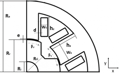
A double salient radial flux SRM is modelled. The basic structure of such machine is presented in Figure 1. The designations of the various parameters are given in the nomenclature section.
The magnetic circuit of the machine is made of SUS410 magnetic stainless steel. Despite its lower magnetic performances, compared to that of iron alloys, this type of material is more suitable for severe environments [1]. However, due to its relatively low permeability, the current levels are higher than those of conventional machines, generating additional thermal constraints to the machine. The shaft is made of steel, and the winding is made of copper (Cu) conductors, supposed to be insulated by a high temperature insulator. The stator and the rotor of the SRM are separated by an irregular air gap.
The variation of the electrical resistivity with the temperature (T) is modeled by the relation (1), where, α is the temperature coefficient [K-1], Tref is a reference temperature, and ρref [Ω.m] is the resistivity at the temperature Tref. For copper, we use: $\alpha =9.93\,\times {{10}^{-3}}[{{K}^{-1}}]$ .
$\rho (T)={{\rho }_{ref}}[1+\alpha (T-{{T}_{ref}})]$ (1)
The modified Frölich-Kennely model, given by (2), is used for the estimation of the variation of the magnetic permeability as a function of the magnetic field (H) and the temperature. In (2), µ0 is the vacuum permeability, while, a, b, and c are temperature dependent parameters.
$\mu (H,T)={{\mu }_{0}}+{{[a+b{{H}^{c}}]}^{-1}}$ (2)
Figure 1. Structure of the modelled SRM
In this work, we have developed continuous functions giving the variations of the parameters a, b and c, as a function of the temperature, based on the experimental values provided in Ref. [1]. These functions are given by Eq. (3), where u(x) represents the Heaviside function, and T is expressed in [℃]. The developed functions fit the experimental data in the way of minimizing the mean of the absolute value of the error.
Figure 2 illustrates the variations of the parameters a, b and c, in normalized values, as a function of the temperature, and Figure 3 shows the first magnetization curves for different temperatures, obtained by introducing (3) into (2).
$\left\{ \begin{matrix} a=132.6u(200-T)+354u(T-200)\left[ 1-{{e}^{\frac{150-T}{100}}} \right]\,\,\,\,\,\,\,\,\,\,\,\, \\ \begin{align} & b=4\left[ u(200-T)+{{e}^{\frac{200-T}{170}}}u(T-200) \right]u(350-T)+ \\ & \,\,\,\,\,\,\,\,\,\,\,u(T-350)\,\left[ 1.68-2.5\,\,{{10}^{-3}}(T-350) \right]\, \\ \end{align} \\ c=0.796u(220-T)+0.953\left[ 1-{{e}^{\frac{20-T}{110}}}u(T-220) \right]\,\,\,\,\,\,\, \\\end{matrix} \right.$ (3)
The parameter “c” representing mainly the saturation bend is only slightly affected by the temperature, while “a” increases and “b” decreases significantly beyond 200℃. The variations of “a” and “b” account for the decrease of the saturation induction of the material.
The heat capacities are assumed to be independent of the temperature, as are the thermal conductivities (λ) of air and that of the insulators. The variations of the thermal conductivities of copper and steel with the temperature are given by (4).
$\left\{ \begin{matrix} {{\lambda }_{Cu}}(T)=401-0.0617[T-273]\, \\ {{\lambda }_{SUS410}}(T)=14+0.012[T-273] \\\end{matrix} \right.$ (4)
Figure 2. Evolution of the parameters a, b and c, in normalized values, as a function of temperature (Experimental data in dotted lines)
Figure 3. B(H) curves for different temperatures
A two-dimensional numerical approach is developed. The magnetic and thermal properties are assumed to be isotropic, and vary non-linearly with the magnetic field and/or the temperature. The variations of the electromagnetic and thermal properties of materials with the temperature are only updated by regions. This makes it possible to decouple the spatial discretization of the magnetic and thermal problems.
A current supply is considered. In Cartesian coordinate system, the magnetic problem is formulated by a two-dimensional magnetostatic model, as function of the magnetic vector potential, given by (5), where ${{\partial }_{x}}$ and ${{\partial }_{y}}$represent the derivatives in the x and y directions,${{A}_{z}}$and ${{J}_{z}}$ are the z components of the magnetic vector potential and the source current density, respectively, and $\mu (H,T)$ is the magnetic permeability depending on the magnetic field H and the temperature T.
${{\partial }_{x}}(\tfrac{1}{\mu (H,T)}{{\partial }_{x}}{{A}_{z}})+{{\partial }_{y}}(\tfrac{1}{\mu (H,T)}{{\partial }_{y}}{{A}_{z}})=-{{J}_{z}}$ (5)
The Joule losses in the conductors are evaluated by the Ohm's law: $p(T)=\rho (T)\,{{J}^{2}}\,[W.\,{{m}^{-3}}]$, and the iron losses can be evaluated by using the specific losses, knowing the distribution of the magnetic field for each position of the rotor [2-4]. In this work, only the Joule losses in the conductors are considered.
The electromagnetic losses are introduced into the thermal model as a heat source, for the transient thermal analysis, in order to obtain the distribution of the temperature in the machine, and its evolution over time. The heat diffusion in the machine is governed by the Eq. (6), where, λ, ρm, Cp, h and Te, are, respectively, the thermal conductivity in [W.m-1.K-1], the mass density in [kg.m-3], the heat capacity in [J.kg-1.K-1], the convection exchange coefficient in [W.m-2.K-1], and the temperature of the external medium.
$\left\{ \begin{matrix} {{\rho }_{m}}{{C}_{p}}{{\partial }_{t}}T={{\partial }_{x}}(\lambda (T){{\partial }_{x}}T)+{{\partial }_{y}}(\lambda (T){{\partial }_{y}}T)+p(T) \\ -\lambda (T){{\partial }_{n}}T=h(T-{{T}_{e}})\,\,\,\,\,\,\,\,\,\,\,\,\,\,\,\,\,\,\,\,\,\,\,\,\,\,\,\,\,\,\,\,\,\,\,\,\,\,\,\,\,\,\,\,\,\,\,\,\,\,\,\,\,\,\,\,\,\,\,\, \\\end{matrix} \right.$ (6)
The heat extraction by a cooling fan could be considered in a simple way, by introducing a negative power into the diffusion Eq. (6). Moreover, the 2D thermal model can be completed by a lumped parameters model, in order to take into account the variation of the temperature along the axis of the machine, by introducing the joule losses in the coils heads [5].
Obtaining convective heat exchange coefficients is a major difficulty in the thermal modeling of electrical machines. They depend on the nature of the fluid flow (laminar or turbulent) and on the roughness of the exchange surfaces. The convection coefficient in the air gap of the studied SRM is one of the most complicated to determine given the doubly salient structure of the machine. In the case of a turbulent regime, it has been shown that the heat transfer in the air gap can be modeled by an equivalent conductive exchange, characterized by an effective thermal conductivity (λeff), calibrated so as to best match the calculated temperatures with measurements [2, 3]. In Ref. [2], the authors chose an effective thermal conductivity of 2W.m-1.K-1 for a rotation speed of 6000 rpm. Given that this effective conductivity is proportional to the square root of the Reynolds number [3], and therefore, to the square root of the speed of rotation, in our case, for a speed of 1500 rpm, we set its value to 1W.m-1.K-1. The external thermal convection coefficients are evaluated by the empirical formulas given in Ref. [4]. The outer surface (S) consists of axial aluminum cooling fins. The effect of the cooling fins is considered by the introduction of an equivalent convection coefficient, increased by the ratio of the surface of the fins to the surface at the outer radius of the stator.
Figure 4. The modeling procedure
The strategy proposes to solve, in an iterative and sequential way, the magnetostatic and the thermal models, as shown in Figure 4. At each iteration, the magnetic model evaluates the magnetic field repartition, the torque and the electromagnetic losses according to the properties of the materials at a given temperature. The electromagnetic losses are then used as a heat source in the thermal model, in order to calculate the new temperature distribution. The properties of the materials are then reassessed, by regions, according to the new temperatures, and then, the electromagnetic quantities are recalculated again. The operation is repeated until the temperature reaches its steady state value in the machine. The initial temperature of the SRM is set to that of the ambient environment.
We considered a 6/4 double salient SRM, whose parameters are given in Table 1. For the numerical implementation of the magneto-thermal problem, we used the magnetic and thermal modules of the Finite Element Method Magnetics “FEMM” free software, driven via MATLAB, thanks to the OctaveFEMM interface [15].
The time step in the temporal resolution of the thermal model is chosen to be very large compared to the electric period. The Joule losses in the three phases are then considered simultaneously.
In the FEMM thermal module, we start by solving the thermal problem without Joule losses in the coils, in order to initialize the temperature in the machine at room temperature. The solution is used as an initial condition for the transient thermal problem in FEMM. To put the machine in severe thermal conditions, the room temperature is set to 363K. These conditions could, for example, correspond to the working of the SRM next to an internal combustion engine (ICE) in a hybrid propulsion.
Table 1. Parameters specification
|
Geometry and specifications |
||||
|
Re=140mm, Rr=79mm, Ri=40mm, Rri=59.25mm, e=1mm, Wc=16mm, hc=33mm, Ws=42mm, Wr=1.3×Ws, d=1mm, hs=36mm, βs=30°, βr=35°, Axial length: L=100mm |
||||
|
Rotation speed, ω (rpm) |
1500 |
|||
|
Electrical current density in the windings, J (A.m-2) |
6×10⁶ |
|||
|
Airgap equivalent thermal conductivity (W.m-1.K-1) |
1 |
|||
|
External convective exchange coefficient (W.m-2.K-1) |
30 |
|||
|
Thermal properties of the used materials at 20℃ |
||||
|
Material |
λ (W.m-1. K-1) |
Cp (J.kg-1.K-1) |
ρm(kg.m-3) |
|
|
SUS410 |
15 |
500 |
7650 |
|
|
Air |
0.0181 |
104 |
1.184 |
|
|
Cu |
401 |
385 |
8954 |
|
|
Al |
236 |
897 |
2707 |
|
|
Steel |
62 |
444 |
7850 |
|
The simulation is performed over 60,000 seconds, with a step of 3,000 seconds. Figure 5 shows the distribution of the temperature in the different regions of the machine, at the end of the simulation. In order to take into account the temperature variation of the air surrounding the machine, the boundary condition imposing the room temperature is applied on an external contour surrounding an air region around the machine. In this case, the temperature Te in Eq. 6 changes over time. At each iteration, the value of Te calculated previously is used.
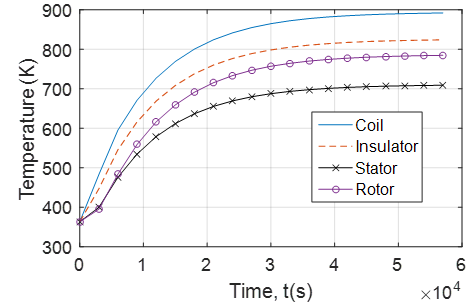
Figure 6 shows the evolution of the Joule losses over time. This evolution follows that of the coils’ resistance. Figure 7 shows the time evolution of the average temperatures in the different regions of the machine. The presence of electrical insulation widens the temperature difference between the coils and the rest of the machine, and probably increases the Joule losses in the coils. In the beginning, the stator and rotor temperatures show the same evolution, and then the rotor temperature increases more than that of the stator, due to the convective exchange of heat with the surrounding air.
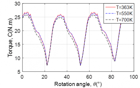
Figure 8 shows the influence of temperature on the torque developed by the machine, at constant current source. We can notice that, for an impressed current, the torque is only slightly affected by the evolution of the temperature, since the salience effect remains important at high temperatures. An abrupt collapse of the developed torque occurs thought for a temperature close to the Curie one. It is the maximum torque that is affected, while the minimum value remains the same. This results in a decrease of the mean torque, and a slight decrease of the torque ripple of the machine. However, the voltage and the speed would be strongly affected by the decrease of the permeability of the magnetic circuit, and the increase of the windings’ resistance, leading to an increase of the voltage drop in the machine. The Joule losses in the windings are multiplied by four; the efficiency of the machine is thus considerably decreased, even though the iron losses may slightly decrease do to the increase of the magnetic circuit resistance and the decrease of the magnitude of the magnetic field. For a study of the power variation of the machine, it is necessary to consider a voltage supply, with a coupling to the circuit equations [6].
Figure 5. The steady state temperature distribution in the different regions of the SRM
Figure 6. Time evolution of the Joule losses in a coil
Figure 7. Time evolution of the temperature in the different regions of the machine
Figure 8. Torque developed by the machine for different values of the rotor temperature
This work proposes a simplified and rapid magneto-thermal modeling of a switched reluctance electric machine operating at high temperatures. The non-linearity of the magnetic and thermal properties are taken into account. The chosen specifications do not correspond to a particular application; the choice only aims to put the machine in harsh thermal conditions.
One of the difficulties encountered in such modeling is the adequate choice of the properties of the materials and their evolution with the temperature. An effort has thus also been made in this direction to provide realistic parameters of the machine, and their integration into the numerical modeling.
Only the Joule losses in the windings are considered as a heat source, considering that the iron losses do not increase, but even slightly decrease with the temperature. The variation of the temperature in the axial direction of the machine, considering the losses in the coils’ heads, could also be integrated into the modeling in a simple manner, by coupling the 2D FEM modeling with a lumped parameters thermal model in the axial direction.
The results show the robustness of the SRM against the temperature increase. Indeed, even though the efficiency is decreased, the developed torque is only slightly affected bellow the Currie temperature. Such machines are thus suitable for harsh environments, such as geothermal fluid pumping for example.
Finally, the approach is mainly theoretical, and experimental validation is needed to appreciate its accuracy, in particular for the thermal part for which the two-dimensional approach is questionable. Nevertheless, the adequate choice of the different parameters, based on theoretical data and measurements, makes it quite realistic.
|
a, b, c |
Modified Frölich-Kennely model parameters |
|
Az |
Z component of the magnetic vector potential [Wb/m] |
|
B |
Magnetic flux density [T] |
|
Cp |
Heat capacity (J.kg-1.K-1) |
|
d |
Distance between the coils and the stator teeth [m] |
|
e |
Smallest airgap [m] |
|
H |
Magnetic field [A/m] |
|
h |
External convective exchange coefficient (W. m-2.K-1) |
|
hc |
Coils' length [m] |
|
hs |
Stator teeth length [m] |
|
Jz |
Z component of the current density [A/m2] |
|
L |
Machine axial length [m] |
|
Re |
Outer radius of the machine [m] |
|
Ri |
Shaft radius [m] |
|
Rr |
Outer rotor radius [m] |
|
Rri |
Inner rotor radius [m] |
|
T |
Temperature [K] |
|
Tref |
Reference Temperature [K] |
|
u |
Heaviside function |
|
Wc |
Coils width [m] |
|
Ws |
Stator teeth width [m] |
|
Wr |
Rotor teeth width [m] |
|
Greek symbols |
|
|
α |
Temperature coefficient [K-1] |
|
$\beta_{s}$ |
Stator teeth opening angle $\left[{ }^{\circ}\right]$ |
|
$\beta_{\mathrm{r}}$ |
Rotor teeth opening angle $\left[{ }^{\circ}\right]$ |
|
$\lambda$ |
Thermal conductivity (W. m-1.K-1) |
|
$\mu$ |
Magnetic permeability [H/m] |
|
$\mu_{0}$ |
Free space magnetic permeability [H/m] |
|
$\rho$ |
Electrical resistivity [Ω.m] |
|
$\rho_{\mathrm{m}}$ |
Mass density (kg/m3) |
|
$\rho_{ref}$ |
Electrical resistivity at the temperature $T_{ref}$ |
|
$\omega$ |
Rotation speed [rpm] |
[1] Noh, M.D., Gi, M.J., Kim, D., Park, Y.W., Lee, J., Kim, J.W. (2015). Modeling and validation of high-temperature electromagnetic actuator. IEEE Transactions on Magnetics, 51(11): 8003504. https://doi.org/10.1109/TMAG.2015.2450364
[2] Lamghari-Jamal, M.I., Fouladgar, J., Zaim, E.H., Trichet, D. (2006). A magneto-thermal study of a high-speed synchronous reluctance machine. IEEE Trans. Mag., 42(4): 1271-1274. https://doi.org/10.1109/TMAG.2006.871956
[3] Huang, Y., Huang, F., Zhang, Y., Chen, C., Yuan, Y., Luo, J. (2019). Thermal characteristics analysis of single-winding bearingless switched reluctance motor. Progress in Electromagnetics Research M, 86: 59-69. https://doi.org/10.2528/PIERM19072305
[4] Sun, Y.K., Zhang, B., Yuan, Y., Yang, F. (2018). Thermal characteristics of switched reluctance motor under different working conditions. Progress in Electromagnetics Research M, 74: 11-23. https://doi.org/10.2528/PIERM18071301
[5] Ghahfarokhi, P.S., Kallaste, A., Belahcen, A., Vaimann, T., Rassõlkin, A. (2018). Hybrid thermal model of a synchronous reluctance machine. Case Studies in Thermal Engineering, 12: 381-389. https://doi.org/10.1016/j.csite.2018.05.007
[6] Adouni, A., Marques Cardoso, A.J. (2019). Thermal analysis of synchronous reluctance machines-A review. Electric Power Components and Systems, 47(6-7): 471-485. https://doi.org/10.1080/15325008.2019.1602688
[7] Takahashi, N., Morishita, M., Miyagi, D., Nakano, M. (2010). Examination of magnetic properties of magnetic materials at high temperature using a ring specimen. IEEE Trans. Mag., 46(2): 548-551. https://doi.org/10.1109/TMAG.2009.2033122
[8] Chen, J., Wang, D., Cheng, S., Wang, Y., Zhu, Y., Liu, Q. (2015). Modeling of temperature effects on magnetic property of nonoriented silicon steel lamination. IEEE Trans. Mag., 51(11): 2002804. https://doi.org/10.1109/TMAG.2015.2432081
[9] Paya, B., Teixeira, P. (2015). Electromagnetic characterization of magnetic steel alloys with respect to the temperature. 8th International Conference on Electromagnetic Processing of Materials, Cannes, France.
[10] Boehm, A., Hahn, I. (2014). Measurement of magnetic properties of steel at high temperatures. IECON 2014 - 40th Annual Conference of the IEEE Industrial Electronics Society, Dallas, TX, USA, pp. 715-721. https://doi.org/10.1109/IECON.2014.7048579
[11] Chen, J.Q., Chen, Z.H., Wang, D., Wu, L.T., Zheng, X.Q., Birnkammer, F., Gerling, D. (2017). Influence of temperature on magnetic properties of silicon steel lamination. AIP Advances, 7(5): 056113. https://doi.org/10.1063/1.4978659
[12] Kurose, H., Miyagi, D., Takahashi, N., Uchida, N., Kawanaka, K. (2009). 3-D eddy current analysis of induction heating apparatus considering heat emission, heat conduction, and temperature dependence of magnetic characteristics. IEEE Trans. Mag., 45(3): 1847-1850. https://doi.org/10.1109/TMAG.2009.2012829
[13] Jang, J.Y., Chiu, Y.W. (2007). Numerical and experimental thermal analysis for a metallic hollow cylinder subjected to step-wise electro-magnetic induction heating. Applied Thermal Engineering, 27(11-12): 1883-1894. https://doi.org/10.1016/j.applthermaleng.2006.12.025
[14] Rahmatinia, S., Fahimi, B. (2017). Magneto-thermal modeling of biological tissues: A step toward breast cancer detection. IEEE Trans. Mag., 53(6): 1-4. https://doi.org/10.1109/TMAG.2017.2671780
[15] http://www.femm.info/wiki/octavefemm.