Hong Li | Yang Liu* | Rende Qi | Yu Ding
© 2021 IIETA. This article is published by IIETA and is licensed under the CC BY 4.0 license (http://creativecommons.org/licenses/by/4.0/).
OPEN ACCESS
This paper proposes the application of a novel finite control set model predictive control (FCS-MPC) strategy in active power filter (APF). In the process of APF compensating harmonic and reactive power, the traditional single vector model predictive current control (MPCC) has low tracking accuracy to harmonic current, while the multi-vector MPCC has the problems of complex calculation and long calculation time, a new multi-vector MPCC control method has proposed in this paper. Firstly, the harmonic reference value is transformed into d-q coordinate system, according to the sector, the slope is calculated and the action time is obtained. Six new expected vectors are synthesized from six effective vectors and zero vectors. The value function is established to loop and calculate the optimal virtual vector, which is applied to APF. Compared with single vector control and traditional multi-vector control, it has a wider vector action area and faster calculation speed. The compensation results and dynamic performance are improved. The simulation results show that the total harmonic distortion (THD) is low.
active power filter (APF), model predictive current control (MPCC), multi-vector, virtual vector
In the daily life of low-voltage power grid and industrial power consumption, a large number of power electronic devices need to be connected. Many power electronic devices have strong nonlinearity. When they are connected to the power grid, they will generate a large number of harmonics and consume reactive power, causing grid pollution and reducing the power quality of the power grid [1-2]. APF is a kind of device which can compensate harmonic and reactive power at the same time. The principle of APF is to inject the detected harmonics in the reverse direction to achieve the purpose of harmonic cancellation [3]. Since APF was put forward, many control methods have appeared [4], including PI control, which is widely used in the traditional industry. However, PI control is difficult to achieve multi-objective control and parameter tuning is difficult to adjust. It has a certain lag through the error feedback adjustment at the current moment, and the industrial environment has certain variability, so it is difficult to adjust PI parameters in real-time [5, 6]. Model predictive control (MPC) is a control method developed from practice to theory with the development of industry, including dynamic matrix control (DMC), model algorithm control (MAC), generalized predictive control (GPC), etc. with the development of microprocessors, model predictive control (MPC) has been widely used in power electronics and converters [6-8]. General power electronic devices have strong nonlinearity, and limited switching state [9, 10]. Jose Rodriguez et al, proposed the finite set model predictive control (FCS-MPC) [10], using the value function to select the optimal switch combination, corresponding to the traditional continuous set model predictive control. However, the traditional FCS-MPC has the problem of on-line calculation, and the switching frequency is not fixed [7-11].
For the problems existing in the control method of FCS-MPC, many scholars in related fields have proposed different improved control methods based on FCS-MPC [6, 10, 11, 12]. Studies [13] have looked at a model predictive control method with time-delay compensation is proposed. The reference current is predicted by Lagrange interpolation. In the future, multiple prediction periods are calculated. Due to the irregular and rapid variation of harmonics, the prediction corresponding to the predicted reference value has a large error at the change. Previous work [14] has pointed out that FCS-MPC was applied to APF, to control APF to compensate harmonic current and reactive power. However, the inherent shortcomings of FCS-MPC were not improved, and vector coverage of all sectors could not be achieved, which affected the control accuracy and compensation results. In the three-phase coordinate system, there are some accumulated errors in the control. The studies [15] describe a multi-vector MPCC is proposed, which takes the mathematical prediction model of d-q as the control object , calculates the action time, and then composes six expected vectors to be selected, and loop the vectors to obtain the vector with the minimum value function, and acts on the APF in turn through the action time [16]. This method can cover all the vectors in six sectors and loop the expected vector directly, which reduces the control delay and improves the compensation accuracy. The calculation of action time and its application in APF fixes the switching frequency and makes up for the inherent shortcomings of FCS-MPC [17, 18].
In this paper, the control equations of APF and APF are established based on APF. The detected harmonics are used as reference current to calculate the vector action time, and six expected vectors with adjustable amplitude and direction covered by the whole sector are synthesized to limit the switching frequency of APF in the period. Then, the value function is established and the expected vector with the minimum error is selected to make the output of APF keep a small error of harmonic reference, while keeping the APF working, the current ripple can be reduced as much as possible. Finally, the simulation model of APF and the algorithm is established to verify its effectiveness and feasibility.
The MPC control method relies on the model of the APF system to predictive how the possible control actions would affect its response. So, the action that is expected to minimize a certain cost function is applied and the process is sequentially repeated. To obtain good control performance when this method is applied to APF, the appropriate model of APF is needed [18, 19].
Figure 1 shows the system main structure of a parallel APF, where ea, eb, ec are grid voltage, ica, icb, icc are the output compensation current of APF, iLa, iLb, iLc are load current, where L and R are the filter inductance and equivalent resistance, C is DC side capacitance, which stores energy for bidirectional flow of APF and grid energy, for Udc of the DC voltage hold stability.
Figure 1. Three-phase parallel APF structure diagram
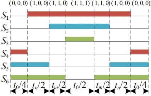
Three groups of switches $S_{x} \in\left\{S_{a}, S_{b}, S_{c}\right\}$ are defined as two states: on and off. To prevent simultaneous conduction failure, dead zone protection is added to the output switch. These switches are defined as Eq. (1).
${{S}_{a}}=\left\{ \begin{align} & 1;\quad \,\text{if}\ {{S}_{1}}\,\text{is}\ \operatorname{ON}\ \text{and}\ {{S}_{4}}\ \text{is}\ \operatorname{OFF} \\ & \text{0};\quad \text{if}\ {{S}_{1}}\,\text{is}\ \operatorname{OFF}\ \text{and}\ {{S}_{4}}\ \text{is}\ \operatorname{ON} \\ \end{align} \right.$
${{S}_{b}}=\left\{ \begin{align} & 1;\quad \,\text{if}\ {{S}_{2}}\,\text{is}\ \operatorname{ON}\ \text{and}\ {{S}_{5}}\ \text{is}\ \operatorname{OFF} \\ & \text{0};\quad \text{if}\ {{S}_{2}}\,\text{is}\ \operatorname{OFF}\ \text{and}\ {{S}_{5}}\ \text{is}\ \operatorname{ON} \\ \end{align} \right.$ (1)
${{S}_{c}}=\left\{ \begin{align} & 1;\quad \,\text{if}\ {{S}_{3}}\,\text{is}\ \operatorname{ON}\ \text{and}\ {{S}_{6}}\ \text{is}\ \operatorname{OFF} \\ & \text{0};\quad \text{if}\ {{S}_{3}}\,\text{is}\ \operatorname{OFF}\ \text{and}\ {{S}_{6}}\ \text{is}\ \operatorname{ON} \\ \end{align} \right.$
Therefore, the overall APF can be in eight (23) possible switch configurations, and the point N are calculated by multiplying the DC link voltage with the state of the respective leg:
${{v}_{aN}}={{S}_{a}}\cdot {{v}_{dc}}$
${{v}_{bN}}={{S}_{b}}\cdot {{v}_{dc}}$ (2)
${{v}_{cN}}={{S}_{c}}\cdot {{v}_{dc}}$
It is necessary to subtract the common-mode voltage vnN needs from (2) to obtain the effective voltage applied to each phase (from points a, b and c to n). The common mode voltage can be simply calculated by considering Kirchhoff's voltage law:
${{v}_{nN}}=\frac{{{v}_{aN}}+{{v}_{bN}}+{{v}_{cN}}}{3}$ (3)
Therefore, the effective phase voltage can be obtained:
${{v}_{an}}={{v}_{aN}}-{{v}_{nN}}$
${{v}_{bn}}={{v}_{bN}}-{{v}_{nN}}$ (4)
${{v}_{cn}}={{v}_{cN}}-{{v}_{nN}}$
Assuming three-phase symmetry, according to the delay of Eq. (5), the output of APF can be defined as Eq. (6), where vaN, vbN, and vcN are the voltages of each phase relative to N point.
$\text{a}={{e}^{j2\pi /3}}=-\frac{1}{2}+j\frac{\sqrt{3}}{2}$ (5)
$\text{v}=\frac{2}{3}({{v}_{aN}}+\text{a}{{v}_{bN}}+{{\text{a}}^{2}}{{v}_{cN}})$ (6)
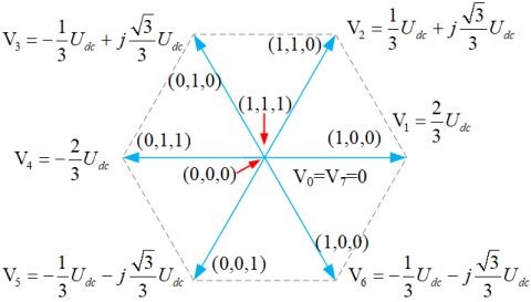
The vector composed of Sx in different switching states of three-phase two-level APF, by applying the complex Clark transformation (1) to (8) for eight possible switch configurations, the input vectors can be shown in Figure 2.
Figure 2. Three-phase two-level parallel APF switch vector in the complex α-β frame
2.1 Discrete mathematical model of three-phase APF
In the three-phase static coordinate system, assuming the three-phase symmetry, according to Kirchhoff's current law, the dynamic expression of Eq. (7) can be obtained, where uca, ucb, and ucc are the output voltage of APF [20].
$\left\{ \begin{align} & L\frac{\text{d}{{i}_{a}}}{\text{d}t}={{e}_{a}}-R{{i}_{a}}-{{u}_{c}}_{a} \\ & L\frac{\text{d}{{i}_{b}}}{\text{d}t}={{e}_{b}}-R{{i}_{b}}-{{u}_{c}}_{b} \\ & L\frac{\text{d}{{i}_{c}}}{\text{d}t}={{e}_{c}}-R{{i}_{c}}-{{u}_{c}}_{c} \\ \end{align} \right.$ (7)
According to Eq. (7), the state variable is set as X=[ia;ib;ic] and the input is U = [ea-uca; eb-ucb; ec-ucc], and the state space model of three-phase two-level APF is established.
$\mathbf{\dot{X}}={{\mathbf{A}}_{3\times 3}}\mathbf{X}+{{\mathbf{B}}_{3\times 3}}\mathbf{U}$ (8)
A and B are state matrix and input matrix, which are determined by model parameters of APF. Among,
$\mathbf{A}=\{{{(-\frac{R}{L})}_{ii}}\},\mathbf{B}=\{{{(\frac{1}{L})}_{ii}}\},i=1,2,3$ (9)
By transforming it into d-q coordinate system and discretizing it, we can get Eq. (10):
$\mathbf{\tilde{X}}(k+1)={{\mathbf{\tilde{\Psi }}}_{2\times 2}}\mathbf{\tilde{X}}(k)+{{\mathbf{\tilde{\Theta }}}_{2\times 2}}\mathbf{\tilde{U}}$ (10)
where,
$\mathrm{\tilde{X}}={{C}_{dq}}{{C}_{32}}\mathbf{X};\mathrm{\tilde{U}=}{{C}_{dq}}{{C}_{32}}\mathbf{U}$ (11)
$\mathbf{\tilde{\Psi }}={{\operatorname{e}}^{\mathbf{\Psi }{{T}_{s}}}};\mathbf{\tilde{\Theta }}=({{\operatorname{e}}^{\mathbf{\Psi }{{T}_{s}}}}-\mathbf{I}){{\mathbf{\Psi }}^{-1}}\mathbf{\Theta }$ (12)
$\begin{align} & \mathbf{\Psi }=\left[ \begin{matrix} -\frac{R}{L} & 0 \\ 0 & -\frac{R}{L} \\\end{matrix} \right],\mathbf{\Theta }=\left[ \begin{matrix} \frac{1}{L} & {} \\ {} & \frac{1}{L} \\\end{matrix} \right] \\ & {{C}_{dq}}=\sqrt{\frac{2}{3}}\left[ \begin{matrix} \sin \omega t & -\cos \omega t \\ -\cos \omega t & -\sin \omega t \\\end{matrix} \right] \\ \end{align}$
${{C}_{32}}=\sqrt{\frac{2}{3}}\left[ \begin{matrix} 1 & -\frac{1}{2} & \frac{1}{2} \\ 0 & \frac{\sqrt{3}}{2} & -\frac{\sqrt{3}}{2} \\\end{matrix} \right]$ (13)
Eq. (10) is the discrete mathematical model in d-q coordinate system, in (12), the TS is the sampling period of the system, in (13), the ꞷ is the phase angle detected by PLL.
2.2 Calculation of reference current
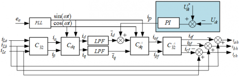
Figure 3. ip-iq method for harmonic detection of the reference current
When APF is used to compensate harmonic and reactive power, it must be detected first, including FFT, FBD, PQ method, and so on. At present, the most widely used ip-iq detection method proposed by H. Akagi is that the fundamental wave of load current is obtained by filtering, and the harmonic content of load current can be obtained by subtracting the load current [21]. The DC side capacitor voltage of APF is controlled by PI, and the compensation part is injected to keep the energy interaction between AC measurement and DC side and stabilize it at the reference value [22, 23]. It has better dynamic performance and tracking performance, and the specific principle is shown in Figure 3.
The detected three-phase harmonics iah, ibh and ich are taken as reference values, it is Xref = [iah;ibh;ich]. In the harmonic detection link, there is a certain time delay from current detection to harmonic calculation, and it cannot be used as the reference value of the predicted value at the next moment. The reference value can be predicted by Lagrange interpolation, and Eq. (14) can be obtained. The error of second-order interpolation and third-order interpolation is small, in order to reduce the amount of calculation, n = 2 is adopted in this paper.
${{\mathbf{\tilde{X}}}_{ref}}(k+1)=\sum\limits_{i=0}^{n}{{{(-1)}^{n-i}}\frac{(n+1)!}{i!(n+1-i)!}\cdot {{\mathbf{X}}_{ref}}(k+i-n\,)\ }$ (14)
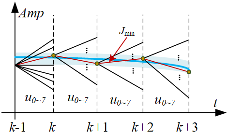
The principle of FCS-MPC is shown in Figure 4.
Figure 4. FCS-MPC principal diagram
In the traditional model predictive current control, a single vector is used in the inner loop control. The value function of subtracting the predicted value from the reference current value in d-q coordinate system is established. In Eq (15), the vector with the minimum J is obtained by traversing from V0 to V6,also simultaneously keeps track of several other objectives can be formulated as follows:
$J=\left( \left. {{\left\| {{C}_{dq}}{{C}_{32}}{{{\mathbf{\tilde{X}}}}_{ref}}(k+1)-\mathbf{\tilde{X}}(k+1) \right\|}_{Q}}+{{h}_{\lim }}(i)+{{\gamma }_{i}}{{s}^{2}}(i) \right) \right.$ (15)
where, Q is the weight matrix, and the tracking weight coefficients of d-axis and q-axis are respectively,hlim(i) imposes the current constraint, while e2(i) penalizes the switching effort which can be controlled by the associated weighting factor g. There terms are defined as follows:
$Q=\left[ \begin{matrix} {{\lambda }_{d}} & {} \\ {} & {{\lambda }_{q}} \\\end{matrix} \right]$ (16)
${{h}_{\lim }}(i)=\left\{ \begin{align} & 0,\ \operatorname{if}i(k+1)\le {{i}_{\max }} \\ & \infty ,\ \operatorname{if}i(k+1)>{{i}_{\max }} \\ \end{align} \right.$ (17)
and
$s(i)=\sum{\left| {{i}_{a,b,c}}(k+1)-{{i}_{a,b,c}}(k) \right|}$ (18)
Through all the vector cycles, Jmin is obtained and the corresponding voltage vector is obtained. The reference harmonic current can be tracked by applying the switching state to APF. This method has a single vector and cannot cover any vector direction of any sector. The optimal switch group obtained by the value function is only limited to the optimal set, that is, there is a certain tracking error. The irregularity of harmonic variation will make the switching frequency change not fixed, which makes the filter design difficult.
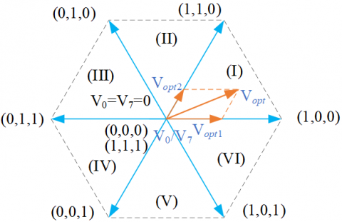
Multi-vector MPCC is a control method based on the optimal duty cycle model [15], the specific principle is shown in Figure 5. The traditional multi-vector MPCC control obtains the optimal vector Vopt1 through the calculation of first loop the vectors, then, the suboptimal voltage vector vopt2 is selected to calculate the time of vector action, the other suboptimal voltage vector Vopt2 is selected to calculate the time of vector action. Finally, the corresponding modulation pulse is output to APF and this style reduces the switching frequency.
In this paper, another multi-vector MPCC strategy is used for three-phase two-level APF, that is, two adjacent vectors and one zero vector are selected in six sectors, six virtual vectors V1d~V6d with adjustable amplitude and direction are synthesized. The value function through the six vectors by calculated online, and the optimal voltage vector is obtained, the principle is shown in Figure 6. The implementation of this method mainly includes three steps: 1) obtain the vector action time, 2) synthesize the expected vector, 3) solve the value function to get the optimal vector.
Figure 5. New multi-vector composite graph
4.1 Calculation of vector action time
The operating time of the voltage vector is obtained by deadbeat error control of d-q axis current change rate. From Eq. (6), the slope of d-q axis under the action of zero vector is Eq. (19).
${{\mathsf{g}}_{\mathsf{0}}}\mathsf{=}\frac{\mathbf{\tilde{X}}(k)-\mathbf{\tilde{X}}(k-1)}{{{T}_{s}}}\left| _{\mathsf{u}=\mathsf{0}} \right.$ (19)
where,
$\mathbf{g}_{0}=\left[\begin{array}{l}g_{0 d} \\ g_{0 q}\end{array}\right], \mathbf{u}=\left[\begin{array}{l}u_{c d} \\ u_{c q}\end{array}\right]$ (20)
If Vn and Vm are two adjacent effective vectors, the d-q axis current slope of these two adjacent effective vectors is Eqns. (21) and (22), and [Vnd;Vnq] and [Vmd;Vmq] are the d-q axis components of Vn and Vm.
${{\mathsf{g}}_{n}}=\frac{\mathbf{\tilde{X}}(k)-\mathbf{\tilde{X}}(k-1)}{{{T}_{s}}}\left| _{\mathsf{u}=\left[ \begin{smallmatrix} {{\operatorname{V}}_{\operatorname{n}d}} \\ {{\operatorname{V}}_{\operatorname{n}q}} \end{smallmatrix} \right]} \right.$ (21)
${{\mathsf{g}}_{m}}=\frac{\mathbf{\tilde{X}}(k)-\mathbf{\tilde{X}}(k-1)}{{{T}_{s}}}\left| _{\mathsf{u}=\left[ \begin{smallmatrix} {{\operatorname{V}}_{\operatorname{m}d}} \\ {{\operatorname{V}}_{\operatorname{m}q}} \end{smallmatrix} \right]} \right.$ (22)
where, [gnd;gnq] and [gmd;gmq] are the slopes of the d-q axis components of vector Vn and Vm, respectively
$\mathbf{g}_{n}=\left[\begin{array}{l}g_{n d} \\ g_{n q}\end{array}\right], \mathbf{g}_{m}=\left[\begin{array}{l}g_{m d} \\ g_{m q}\end{array}\right]$ (23)
According to the principle of dead-beat control, there is no error between the predicted value and the given value at k + 1 time. Therefore, the discrete prediction model (24) can be obtained, tn, tm, to are the action time of the expected vector Vnd, Vmd, and zero vector, the purpose is to predict that the output value is equal to the harmonic reference value, that is, zero error.
${{\mathsf{e}}_{ss}}=\mathbf{\tilde{X}}(k+1)-{{C}_{dq}}{{C}_{32}}{{\mathbf{\tilde{X}}}_{ref}}(k+1)=\mathsf{0}$ (24)
${{\mathsf{e}}_{ss}}=\left[ \begin{align} & {{e}_{ssd}} \\ & {{e}_{ssq}} \\ \end{align} \right]$ (25)
If we combine the above formula, we can get that tn, tm and to are in Eq. (26).
$\begin{align} & {{t}_{n}}=\frac{{{e}_{ssd}}({{g}_{mq}}-{{g}_{0q}})+{{e}_{ssq}}({{g}_{0d}}-{{g}_{md}})}{{{g}_{0d}}({{g}_{nq}}-{{g}_{mq}})+{{g}_{0q}}({{g}_{md}}-{{g}_{nd}})+{{g}_{nq}}({{g}_{nd}}-{{g}_{md}})} \\ & \quad \ +\frac{{{T}_{s}}({{g}_{0q}}{{g}_{md}}-{{g}_{mq}}{{g}_{0d}})}{{{g}_{0d}}({{g}_{nq}}-{{g}_{mq}})+{{g}_{0q}}({{g}_{md}}-{{g}_{nd}})+{{g}_{nq}}({{g}_{nd}}-{{g}_{md}})} \\ \end{align}$
$\begin{align} & {{t}_{m}}=\frac{{{e}_{ssd}}({{g}_{0q}}-{{g}_{nq}})+{{e}_{ssq}}({{g}_{nd}}-{{g}_{0d}})}{{{g}_{0d}}({{g}_{nq}}-{{g}_{mq}})+{{g}_{0q}}({{g}_{md}}-{{g}_{nd}})+{{g}_{nq}}({{g}_{nd}}-{{g}_{md}})} \\ & \quad \ +\frac{{{T}_{s}}({{g}_{0d}}{{g}_{nq}}-{{g}_{0q}}{{g}_{nd}})}{{{g}_{0d}}({{g}_{nq}}-{{g}_{mq}})+{{g}_{0q}}({{g}_{md}}-{{g}_{nd}})+{{g}_{nq}}({{g}_{nd}}-{{g}_{md}})} \\ \end{align}$ (26)
${{t}_{0}}={{T}_{s}}-{{t}_{n}}-{{t}_{m}}$
In all sectors, when the APF output tracks the reference harmonic current, if the vector action time is too long or the sampling period Ts is small enough, there may be two effective vectors whose action time is longer than the sampling period. here,
$t_{n}^{*}=\frac{{{t}_{n}}}{{{t}_{n}}+{{t}_{m}}}{{T}_{s}}$
$t_{n}^{*}=\frac{{{t}_{m}}}{{{t}_{n}}+{{t}_{m}}}{{T}_{s}}$ (27)
$t_{n}^{*}=0$
4.2 Composite expected virtual vector
As shown in Figure 6, the expected virtual vector is composed of two adjacent effective vectors and a zero vector, so six expected virtual vectors are synthesized in the I ~ VI sector respectively, and then the optimal virtual vector can be obtained by traversing the objective function. Assuming that the required virtual vector is VD, then according to the action time of two adjacent effective vectors and one zero vector, they are combined respectively, as shown in Figure 6.
Figure 6. Virtual vector composition
Figure 7. Expectation vector action diagram
The process of Vd action is shown in Figure 7. The voltage of the resultant expected vector in d-q coordinate system is Eq. (28), and [ucdd,ucdq] is the component of APF expected output voltage in d-q axis.
$\left[ \begin{align} & {{u}_{cdd}} \\ & {{u}_{cdq}} \\ \end{align} \right]=\left[ \begin{matrix} \frac{{{t}_{n}}}{{{T}_{s}}} & {} \\ {} & \frac{{{t}_{n}}}{{{T}_{s}}} \\\end{matrix} \right]\left[ \begin{matrix} {{u}_{nd}} \\ {{u}_{nq}} \\\end{matrix} \right]+\left[ \begin{matrix} \frac{{{t}_{m}}}{{{T}_{s}}} & {} \\ {} & \frac{{{t}_{m}}}{{{T}_{s}}} \\\end{matrix} \right]\left[ \begin{matrix} {{u}_{md}} \\ {{u}_{mq}} \\\end{matrix} \right]$ (28)
4.3 Selection of optimal virtual vector
At this time, the virtual vector is brought in to get the new input, the objective function is the same as Eq. (15), and the objective function is brought in to loop the six expected virtual vectors.
$\left[ \begin{align} & {{u}_{cdd}} \\ & {{u}_{cdq}} \\ \end{align} \right]=\left[ \begin{matrix} \frac{{{t}_{n}}}{{{T}_{s}}} & {} \\ {} & \frac{{{t}_{n}}}{{{T}_{s}}} \\\end{matrix} \right]\left[ \begin{matrix} {{u}_{nd}} \\ {{u}_{nq}} \\\end{matrix} \right]+\left[ \begin{matrix} \frac{{{t}_{m}}}{{{T}_{s}}} & {} \\ {} & \frac{{{t}_{m}}}{{{T}_{s}}} \\\end{matrix} \right]\left[ \begin{matrix} {{u}_{md}} \\ {{u}_{mq}} \\\end{matrix} \right]$ (29)
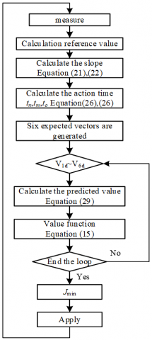
The specific algorithm is shown in appendix 1.
In order to verify the effectiveness and feasibility of this method in APF, the control schematic diagram and analysis as shown in Appendix 2, and its parameters are shown in Table 1.
Table 1. Parameters of simulation model
|
parameter |
value |
|
Grid voltage V/f |
380 V/50 HZ |
|
DC side reference voltage Udc /V |
800 V |
|
Capacitance value C/μF |
3000 μF |
|
Inductance value L/ mH |
4 mH |
|
Resistance value R/Ω |
0.01 Ω |
|
Load resistance value Rload/Ω |
10 Ω |
In order to verify the dynamic performance of the method, the load resistance is set to change to 3.75 Ω in 0.4 s.
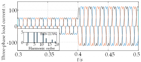
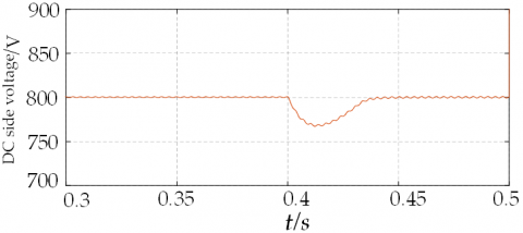
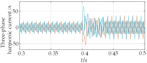
In Figure 8, it’s shown that (a) Description of what the load current with harmonics without compensation; (b) Description of what the result of PI control of DC side capacitor voltage; (c) Description of what the three-phase harmonics detected by ip-iq method in Figure 3
The load in simulation is connected resistance load of an uncontrolled diode rectifier, as shown in Figure 8(a), the harmonics are mainly low order harmonics such as 5, 7, 11, 13, and the total harmonic distortion (THD) rate is 22.76%, which is higher than the standard of THD = 5% for the low-voltage power grid. (b) is what the DC side capacitor voltage was controlled by PI control, and then the dynamic diagram of load change, we can saw that it has better dynamic performance, but the parameter selection is more difficult. In the actual situation, the device parameters change, it is difficult to achieve the optimal, which is also the disadvantage of PI control. (c) Description of what the three-phase harmonics have detected by ip-iq method in Figure 3, the harmonic content is high.
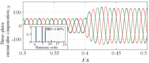
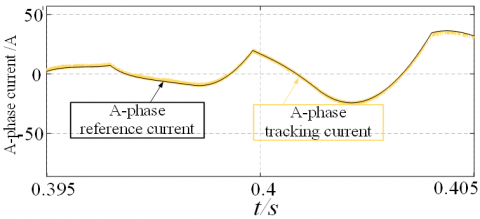
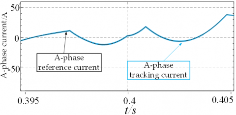
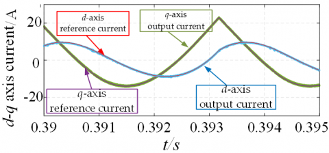
In Figure 9, it’s shown that (a) Description of what the three-phase load current after compensation; (b) and (c) Description of what the accuracy of tracking reference A-phase current; (e) and (f) Description of what the accuracy of tracking reference d-q axis current; (d) Description of what the THD variation of two control methods.
Figure 9 shows the main purpose of the algorithm, the compensation and tracking the performance of harmonics. (a) shows the three-phase network current after compensation, the harmonic content was significantly reduced, and the THD = 1.86%. The APF, as a harmonic source, has low content of 3, 9, 15 harmonics, Compensation result displays the algorithm has good compensation ability to control APF. (b) and (c) shows that single phase of APF tracks A-phase harmonic in the three-phase coordinate system. Be relative to the traditional method, the algorithm shows good convergence and a small error in the three-phase coordinate system through tracking in d-q coordinate system. (c) and (d) description of what tracking compensation in d-q coordinate system. shows the comparison of the traditional control, the control effect of the method in this paper can keep the grid current distortion rate lower.
The simulation results showed that the algorithm is effective and feasible, and also has the dynamic performance of fast-tracking. When the load changes, it can compensate for the harmonic in time and reduce the current ripple. The multi-vector MPCC method can show better tracking effect because it can cover all sectors, and the switching frequency conversion times are fixed in each cycle, which reduces the device loss and improves the shortcomings of the traditional FCS-MPC.
(a) Load current
(b) DC side voltage
(c) Three-phase harmonic
Figure 8. The harmonics without compensation, DC side capacitor voltage, and the three-phase harmonics
(a) The current based on novel method
(b) Traditional method in A-phase
(c) Novel method in A-phase
(d) Traditional method in d-q coordinate system
(e) Novel method in d-q coordinate system
(f) The comparison of two methods
Figure 9. the three-phase load current after compensation, the accuracy of tracking reference, and THD variation
In this paper, the three-phase two-level APF is taken as the control object, and the application of multi-vector MPCC in tracking and compensating harmonic current generated by nonlinear load is studied. By synthesizing six virtual expected vectors with adjustable size and direction from two effective vectors and one zero vector, this method has the accurate tracking effect, fast traversal calculation, and reduces the computational burden of the system. When the load changes, the tracking performance can be maintained all the time, and the tracking error is small throughout the whole process, which improves the control accuracy. A new method was compared with the traditional control method, it can maintain lower THD and improve the performance of APF. The looping optimization is an important part of FCS-MPC, this method combines two directions of simplified optimization process and adjacent candidate vectors, which is proved theoretically and can also be proved by constructing the Lyapunov function. It is feasible in practical application, which can reduce the control delay and APF performance.
This work is supported by the National Science Foundation of China (Grant numbers: 61863023).
Appendix 1
Appendix 2
As shown in Appendix 2, the control process includes the following steps:
[1] Singh, B., Al-Haddad, K., Chandra, A. (1999). A review of active filters for power quality improvement. IEEE Transactions on Industrial Electronics, 46(5): 960-971. https://doi.org/10.1109/41.793345
[2] Akagi, H. (1996). New trends in active filters for power conditioning. IEEE Transactions on Industry Applications, 32(6): 1312-1322. https://doi.org/10.1109/28.556633
[3] Garcia-Cerrada, A., Pinzon-Ardila, O., Feliu-Batlle, V., Roncero-Sanchez, P., Garcia-Gonzalez, P. (2007). Application of a repetitive controller for a three-phase active power filter. IEEE Transactions on Power Electronics, 22(1): 237-246. https://doi.org/10.1109/TPEL.2006.886609
[4] Cao, X.D., Dong, K., Wei, X.L. (2020). An improved control method based on source current sampled for shunt active power filters. Energies, 13(6): 1405. https://doi.org/10.3390/en13061405
[5] Daniyal, H., Lam, E., Borle, L.J., Iu, H.H.C. (2011). Hysteresis, PI and ramptime current control techniques for APF: An experimental comparison. 2011 6th IEEE Conference on Industrial Electronics and Applications, Beijing, pp. 2151-2156. https://doi.org/10.1109/ICIEA.2011.5975947
[6] Daniel, W., Ryszard, S. (2007). Sensorless predictive control of three-phase parallel active filter. AFRICON 2007, Windhoek, South Africa, pp. 1-7. https://doi.org/10.1109/AFRCON.2007.440159
[7] Marks, J.H., Green, T.C. (2002). Predictive transient-following control of shunt and series active power filters. IEEE Transactions on Power Electronics, 17(4): 574-584. https://doi.org/10.1109/TPEL.2002.800970
[8] Dragičević, T. (2018). Model predictive control of power converters for robust and fast operation of AC microgrids. IEEE Transactions on Power Electronics, 33(7): 6304-6317. https://doi.org/10.1109/TPEL.2017.2744986
[9] Kouro, S., Cortes, P., Vargas, R., Ammann, U., Rodriguez, J. (2009). Model predictive control-A simple and powerful method to control power converters. IEEE Transactions on Industrial Electronics, 56(6): 1826-1838. https://doi.org/10.1109/TIE.2008.2008349
[10] Rodriguez, J., Kazmierkowskiet, M.P., Espinoza, J.R. et al. (2013). State of the art of finite control set model predictive control in power electronics. IEEE Transactions on Industrial Informatics, 9(2).
[11] Kwak, S., Park, J. C. (2014). Switching strategy based on model predictive control of VSI to obtain high efficiency and balanced loss distribution. IEEE Transactions on Power Electronics, 29(9): 4551-4567. https://doi.org/10.1109/TPEL.2013.2286407
[12] Aguilera, R.P., Lezana, P., Quevedo, D.E. (2015). Switched model predictive control for improved transient and steady-state performance. IEEE Transactions on Industrial Informatics, 11(4): 968-977. https://doi.org/10.1109/TII.2015.2449992
[13] Jin, T., Shen, X.Y., Su, T.X., Flesch, R. (2019). Model predictive voltage control based on finite control set with computation time delay compensation for PV systems. IEEE Transactions on Energy Conversion, 34(1): 330-338. https://doi.org/10.1109/TEC.2018.2876619
[14] Foster, J.G.L., Pereira, R.R., Gonzatti, R.B., Sant’Ana, W.C., Mollica, D., Lambert-Torres, G. (2019). A review of FCS-MPC in multilevel converters applied to active power filters. 2019 IEEE 15th Brazilian Power Electronics Conference and 5th IEEE Southern Power Electronics Conference (COBEP/SPEC), Santos, Brazil, pp. 1-6. https://doi.org/10.1109/COBEP/SPEC44138.2019.9065398
[15] Xu, Y.P., Wang, J.B., Zhang, B.C., Zhou, Q. (2018). Three-vector-based model predictive current control for permanent magnet synchronous motor. Transactions Of China Electrotechnical Society, 33(5). https://doi.org/10.19595/j.cnki.1000-6753.tces.170044
[16] Aguirre, M., Kouro, S., Rojas, C., Rodriguez, J., Leon, J. (2018). Switching frequency regulation for FCS-MPC based on a period control approach. IEEE Transactions on Industrial Electronics, 65(7): 5764-5773. https://doi.org/10.1109/TIE.2017.2777385
[17] Mohapatra, S.R., Agarwal, V. (2018). A low computational cost model predictive controller for grid connected three phase four wire multilevel inverter. 2018 IEEE 27th International Symposium on Industrial Electronics (ISIE), Cairns, QLD, pp. 305-310. https://doi.org/10.1109/ISIE.2018.8433727
[18] Aguilera, R.P., Lezana, P., Quevedo, D.E. (2013). Finite-control-set model predictive control with improved steady-state performance. IEEE Transactions on Industrial Informatics, 9(2): 658-667. https://doi.org/10.1109/TII.2012.2211027
[19] Komurcugil, H., Kukrer, O. (2006). A new control strategy for single-phase shunt active power filters using a Lyapunov function. IEEE Transactions on Industrial Electronics, 53(1): 305-312.
[20] Young, H.A., Perez, M.A., Rodriguez, J. (2016). Analysis of finite-control-set model predictive current control with model parameter mismatch in a three-phase inverter. IEEE Transactions on Industrial Electronics, 63(5):
[21] Akagi, H., Kanazawa, Y., Nabae, A. (1984). Instantaneous reactive power compensators comprising switching devices without energy storage components. IEEE Transactions on Industry Applications, IA-20(3): 625-630. https://doi.org/10.1109/TIA.1984.4504460
[22] Young, H.A., Perez, M.A., Rodriguez, J. (2016). Analysis of finite-control-set model predictive current control with model parameter mismatch in a three-phase inverter. IEEE Transactions on Industrial Electronics, 63(5): 3100-3107. https://doi.org/10.1109/TIE.2016.2515072
[23] Alam, K.S., Xiao, D., Akter, M.P. et al. (2018). Modified MPC with extended voltage vectors for grid-connected rectifier. IET Power Electron, 11(12): 1926-1936. https://doi.org/10.1049/iet-pel.2017.0883