Ayachi Errachdi* | Mohamed Benrejeb
OPEN ACCESS
In this paper, nonlinear observer design for a chaotic system has been investigated. Indeed, a high gain observer and a sliding mode observer are proposed to the Colpitts circuit. The synthesis of these observers took place under certain sufficient conditions arising directly necessary and sufficient conditions established for nonlinear systems. Comparing with the results obtained by these observers, the high gain observer showed a good ability to reconstruct the states of the chaotic system and providing a small mean squared error compared to that of the sliding mode observer.
chaos system, high gain observer, sliding mode observer, Colpitts circuit
Nonlinear systems that under the specific conditions exhibit chaotic behaviour, attracted wide interest of researches in the last several decades [1-3].
Indeed, in Pecora and Caroll [4], a method is developed to realize the chaos synchronization between two identical chaotic systems with different initial conditions, the synchronization of chaotic systems has attracted considerable attention due to its potential applications in many areas, such as chemical reactions, biological systems, information processing, and secure communication.
Majority of the theoretical results concerning chaos synchronization for the most part focal point on systems whose parameters are exactly known in advance. However, in different practical situations, because the structural variations of the process, the real values of parameters of different process cannot be known entirely. Whereas, it is necessary to know the real value of the unknown parameter for practical applications.
For this reason, many efforts have been devoted, in the literature, to the problem of synchronization of chaotic systems and estimation of its unknown parameter. For example, the adaptive impulsive synchronization and estimation of parameters of chaotic systems only by using discontinuous drive signals are investigated in Gao and Hu [5].
The adaptive synchronization scheme and Lyapunov stability theory are used to discuss the complete synchronization, phase synchronization and parameter estimation in Ma et al. [6].
The parameter estimation and the Lyapunov function are used in synchronization between two nonlinear plants is developed by Banerjee and Chowdhury [7].
The parameter estimation for chaotic systems by using the chaotic search artificial bee colony algorithm is proposed by Zhao et al. [8].
The synchronization and parameter identification of chaotic system with unknown parameters and mixed delays are developed by Zhu [9].
The problems of chaotic synchronization for a class of uncertain chaotic systems and chaos-based secure communication based on observer design method, are discussed by Jiang et al. and Alexander et al. [10-11].
The observer-based synchronization of chaotic systems with first-order coder in the presence of information constraints was introduced by Sharma and Kar [12] and using contraction theory by Teh-Lu and Shin-Hwa [13].
The adaptive synchronization problem of the drive–response-type chaotic systems via a scalar transmitted signal is discussed by Dimitriev et al. [14].
This paper investigates, motivated by the above discussion, the High Gain Observer (HGO) and the Sliding Mode Observer (SMO) in order to estimate the state of Colpitts chaotic systems.
For instance, a subsection will be considered at the presentation of the Colpitts device, as well as it treats essentially the observer estimation of the device.
Chaos in the Colpitts oscillator has been reported first by Kennedy [1-3]. Later, the chaotic behavior of this oscillator has been investigated by several authors due to its applications in encryption and modulation methods applied to communication systems [15-22].
The paper is organized as follows. The Colpitts circuit and the problem formulation are presented in section 2. Section 3 and 4 investigate the design state of the high gain observer and the design state of the sliding mode observer of the Colpitts system. Finally, some conclusions are presented in section 5.
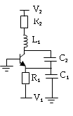
The Colpitts oscillator that we consider is shown in figure 1, is a combination of single bipolar junction Q which is biased in its active region by appropriate choice of R1, an inductor L1 with series resistance R2, a capacitive divider composed of C1 and C2 and V1=V2.
In this paper, the used parameters are L1=100μH, C1=C2=47nF, R1=45Ω.
Figure 1. Circuit diagram of a classical Colpitts oscillator
The Colpitts oscillator, shown in Figure 1, can be described by the following system:
$\left\{ \begin{array}{c}{\dot{x}_{1}(t)=-c x_{3}(t)-c x_{2}(t)-d x_{1}(t)} \\ {\dot{x}_{2}(t)=b x_{1}(t)} \\ {\dot{x}_{3}(t)=-a \exp \left(-x_{2}(t)\right)+a x_{1}(t)+a }\end{array}\right.$ (1)
with x1(t)=IL(t), x2(t)=VC2(t),x3(t)=VC1(t), a=6.2723,b=6.2723 and c=0.0797.
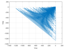
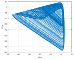
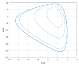
The resistance is bifurcation parameter and route to chaos is period-doubling [1-3]. Time varying of parameter causes change of the system state. In Figures 2, 3 and 4, three cases of R2 are taken (d=R2/L1w ).
Figure 2. Period attractor when d=0.06898
Figure 3. Chaotic attractor when d=0.6898
Figure 4. Period attractor when d=1.6898
From these figures, the system (3) exhibits a chaotic attractor when d= 0.6898 (Figure 3).
For numerical simulations, we take the initial conditions as (x1(0)=0, x2(0)=0,x3(0)=0 ).
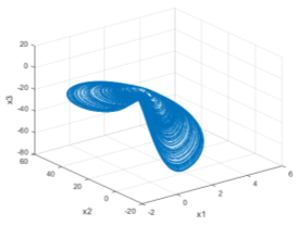
Figure 5 shows the 3-D phase portrait of the Colpitts chaotic system (1).
Figure 5. 3-D chaotic Colpitts circuit
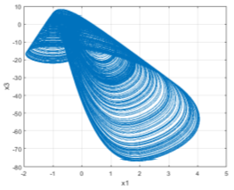
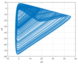
Figures 6, 7 and 8 show the 2-D projections of the Colpitts chaotic system (1) on the (x1, x3), (x2,x3) and (x1,x2) coordinate planes respectively.
Figure 6. 2-D projection of the Colpitts chaotic system on the (x1,x3) plane
Figure 7. 2-D projection of the Colpitts chaotic system on the ( x2, x3) plane
Figure 8. 2-D projection of the Colpitts chaotic system on the (x1,x2) plane
The system (1) can be rewritten in the form:
$\left\{ \begin{array}{l}{\dot{x}(t)=f(x(t), u(t))} \\ {y(t)=g(x(t)), \cdots \cdots \cdots x_{0}=x\left(t_{0}\right)}\end{array}\right.$ (2)
where the state x∈Rn, the input vector is u∈Rm, the output of the system y∈R, nf(.):Rn*Rm→Rn and g(.):Rn*Rm→Rn are locally Lipschitz on x,m≤n.
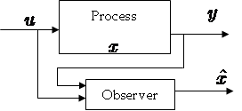
An observer for the system (2) is an auxiliary dynamic system whose inputs are the inputs/output of (2) and the output is the estimated state ${\hat{x}}$, as shown in Figure 9.
Figure 9. The principle of the observer
The observer of the system (2) can be represented as follows:
$\left\{\begin{array}{l}{\dot{\hat{x}}(t)=h(\hat{x}(t), y(t), u(t))} \\ {\hat{y}(t)=C \hat{x}, \ldots \ldots \ldots \ldots \hat{x}_{0}=\hat{x}\left(t_{0}\right)}\end{array}\right.$ (3)
Our objective is to find the estimated state ${\hat{x}}$(t) of x(t) which verify the condition $\lim _{t \rightarrow \infty}\|x(t)-\hat{x}(t)\| \ll \varepsilon, \varepsilon>0$.
In the expression of the system (3), we consider the output function as y=x2, the chaotic system is algebraically observable, the states can be as follows:
$\left\{\begin{aligned} \dot{x}_{1}(t)=\frac{\dot{x}_{2}(t)}{b}=\frac{\dot{y}(t)}{b} \\ \dot{x}_{2}(t)=b x_{2}(t) \\ \dot{x}_{3}(t)=-\frac{1}{c}\left[\frac{1}{b} \ddot{y}(t)+\frac{d}{b} \dot{y}(t)+c y(t)\right] \end{aligned}\right.$ (4)
Thus, in other form:
$\left(\begin{array}{c}{\dot{x}_{1}(t)} \\ {\dot{x}_{2}(t)} \\ {\dot{x}_{3}(t)}\end{array}\right)=\left(\begin{array}{ccc}{-d} & {-c} & {-c} \\ {b} & {0} & {0} \\ {a} & {0} & {0}\end{array}\right)\left(\begin{array}{l}{x_{1}(t)} \\ {x_{2}(t)} \\ {x_{3}(t)}\end{array}\right)$ $+\left(\begin{array}{c}{0} \\ {0} \\ {-a \exp \left(-x_{2}(t)\right)+a}\end{array}\right)$
$y(t)=\left[\begin{array}{ccc}{0} & {1} & {0}\end{array}\right] x(t)$ (5)
with q=3, n=3 and n1=n2=n3=1.
In order to find an observer of the nonlinear system (5), we consider a benchmark system given by:
$\left\{\begin{array}{l}{\dot{x}(t)=A x(t)+F(u(t), x(t))} \\ {y(t)=C x(t)=x^{1}(t)}\end{array}\right.$ (6)
where
$F(x(t), u(t))=\left[\begin{array}{c}{F^{1}\left(x^{1}(t), u(t)\right)} \\ {\vdots} \\ {F^{q-1}\left(x^{1}(t), \ldots, x^{q-1}(t)\right)} \\ {F^{q}(x(t), u(t))}\end{array}\right]$
A is a matrix with dimension p╳p
$A=\left[\begin{array}{cccccc}{0} & {I_{p}} & {0_{p}} & {\cdots} & {\cdots} & {0_{p}} \\ {0_{p}} & {0_{p}} & {\ddots} & {0_{p}} & {\vdots} & {\vdots} \\ {\vdots} & {\vdots} & {0_{p}} & {\ddots} & {\ddots} & {\vdots} \\ {\vdots} & {\vdots} & {\ddots} & {0_{p}} & {\ddots} & {0_{p}} \\ {\vdots} & {\vdots} & {\vdots} & {\ddots} & {0_{p}} & {I_{p}} \\ {0_{p}} & {0_{p}} & {\cdots} & {\cdots} & {0_{p}} & {0_{p}}\end{array}\right]$
x(t)=[x1(t)...xq(t)]T∈Rn
xk(t)=[x1k(t)...xpk(t)]T∈Rp,k=1,...q, the output y(t)∈Rp, the input u(t)∈Rm, F(u(t),x(t)) has a triangular structure with respect to the state x(t) and the matrix has the following particular structure
C=[Ip,Op,...,Op]
where Ip is the p*p identity matrix and Op is the p*p null matrix.
For the nonlinear system (5), the synthesis of such observer certain conditions is necessary. For this reason, some assumptions are cited to consist the design state of observer for system [18].
A1) The input u(t) is bounded. u(t)∈U,t≥0, U is a compact of Rm.
A2) The function F(u(t),x(t)) is globally Lipschitzian with respect to x(t), uniformly in u(t),
A3) Each function Fk(u(t),x(t)) satisfies the following rank condition:
$\operatorname{Rang}\left(\frac{\partial F^{k}(u(t), x(t))}{\partial x^{k+1}}\right)^{T}=n_{k+1} \quad \forall x \in R^{n \circ} ; \forall u \in U$ (7)
moreover $\exists \alpha, \beta>0$ such that for all k∈{1,...,q-1},
$\alpha^{2} I_{n_{k+1}} \leq\left(\frac{\partial F^{k}(u(t), x(t))}{\partial x^{k+1}}\right)^{T} \frac{\partial F^{k}(u(t), x(t))}{\partial x^{k+1}} \leq \beta^{2} I_{n_{k+1}}$ (8)
${{I}_{nk+1}}$ is the identity matrix (nK+1)*(nk+1)
The high gain observer (HGO) for the system (5) can be described by the following dynamic system:
$\dot{\hat{x}}(t)=A \hat{x}(t)+F(u(t), \hat{x}(t))-\theta \Delta_{\theta}^{-1} S^{-1} C^{T} C(\hat{x}(t)-y(t))$ (9)
△θ is the block diagonal matrix defined by $\Delta_{\theta}=\operatorname{diag}\left[I_{p}, \frac{1}{\theta} I_{p}, \cdots, \frac{1}{\theta^{q-1}} I_{p}\right], \theta>0$, θ>0 is a real number, S is the unique solution of the algebraic Lyapunov equation
S+ATS+SA-CTC=0
S is symmetric positive definite. The vector S-1CT is $S^{-1} C^{T}=\left[\begin{array}{ccc}{C_{q}^{1} I_{n_{1}}} & {\dots} & {C_{q}^{q} I_{n_{1}}}\end{array}\right]^{T}$ where $S(i, j)=(-1)^{(i+j)} C_{i+j-2}^{j-2}, \forall \cdot 1 \leq i, j \leq p$, $\forall \cdot 1 \leq i, j \leq p$ and $C_{n}^{p}=\frac{n !}{(n-p) ! p !}$.
Let us consider the following expression of $K\left(\tilde{x}^{1}\right)$:
$K\left(\tilde{x}^{1}\right)=C^{T} C \tilde{x}^{1}=C^{T} C(\hat{x}(t)-x(t))$ (10)
with $\tilde{x}^{1}=\hat{x}-x$, x is the unknown trajectory of system (5).
Thus, the expression (11) becomes as follows:
$\dot{\hat{x}}(t)=A \hat{x}(t)+F(u(t), \hat{x}(t))-\theta \Delta_{\theta}^{-1} S^{-1} K\left(\tilde{x}^{1}(t)\right.$ (11)
with S and its inverse are given as
$S=\left(\begin{array}{ccc}{\frac{1}{\theta}} & {\frac{-1}{\theta^{2}}} & {\frac{1}{\theta^{3}}} \\ {\frac{-1}{\theta^{2}}} & {\frac{2}{\theta^{3}}} & {\frac{-3}{\theta^{4}}} \\ {\frac{1}{\theta^{3}}} & {\frac{-3}{\theta^{4}}} & {\frac{6}{\theta^{5}}}\end{array}\right) ; S^{-1}=\left(\begin{array}{ccc}{3 \theta} & {3 \theta^{2}} & {\theta^{3}} \\ {3 \theta^{2}} & {5 \theta^{3}} & {2 \theta^{4}} \\ {\theta^{3}} & {2 \theta^{4}} & {\theta^{5}}\end{array}\right)$
θ>0 is a real number and $K(\tilde{x})$ is given by
$S^{-1} C^{T}=\left(\begin{array}{c}{3 \theta} \\ {3 \theta^{2}} \\ {\theta^{3}}\end{array}\right)$ (12)
Then, we obtain the equation of the high gain observer of the system class (5), in the following form:
$\dot{\hat{x}}(t)=f(u(t), \hat{x}(t))+\left(\begin{array}{c}{3 \theta} \\ {3 \theta^{2}} \\ {\theta^{3}}\end{array}\right)(\hat{x}(t)-x(t))$ (13)
The equations making the high gain observer are:
$\left\{\begin{array}{l}{\dot{\hat{x}}_{1}=-c \hat{x}_{3}-c \hat{x}_{2}-d \hat{x}_{1}+3 \theta\left(x_{1}-\hat{x}_{1}\right)} \\ {\dot{\hat{x}}_{\hat{x}_{2}}=b \hat{x}_{1}+3 \theta^{2}\left(x_{2}-\hat{x}_{2}\right)} \\ {\dot{\hat{x}}_{3}=a \hat{x}_{1}-a \exp \left(-\hat{x}_{2}\right)+a+\theta^{2}\left(x_{3}-\hat{x}_{3}\right)}\end{array}\right.$ (14)
or $x_{1}=\frac{\dot{y}}{b}$ and $x_{3}=-\frac{1}{c}\left[\frac{1}{b} \ddot{y}+\frac{d}{b} \dot{y}+c y\right]$, so the system can be rewritten as follows
$\left\{\begin{array}{l}{\hat{x}_{1}=-c \hat{x}_{3}-c \hat{x}_{2}-d \hat{x}_{1}+\frac{3}{b} \theta^{2}\left(y-\hat{x}_{2}\right)} \\ {\hat{x}_{2}=b \hat{x}_{1}+3 \theta\left(x_{2}-\hat{x}_{2}\right)} \\ {\hat{x}_{3}=a \hat{x}_{1}-a \exp \left(-\hat{x}_{2}\right)+a+\left(\frac{\theta^{3}}{b c}-\frac{3 d}{b c} \theta^{2}-3 \theta\right)\left(x_{3}-\hat{x}_{2}\right)}\end{array}\right.$ (15)
For all simulation, η=1, the used value of θ is 100 and the initial conditions of the high gain observer are ($\left(\hat{x}_{1}(0)=2.1, \hat{x}_{2}(0)=-0.1, \cdot \widehat{x}_{3}(0)=1.506\right)$).
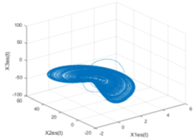
Figure 10 shows the 3-D phase portrait of the Colpitts chaotic system (15) using the high gain observer.
Figure 10. 3-D high gain observer of chaotic Colpitts circuit
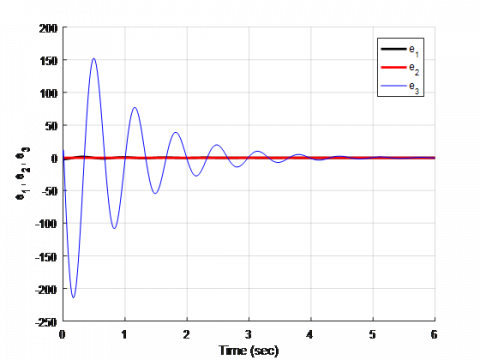
The Figure 11 illustrate the time evolution of the estimation error e1, e2 and e3 using the high gain observer.
Figure 11. Time evolution of the estimation errors
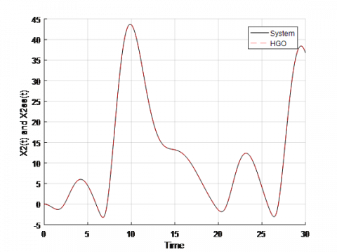
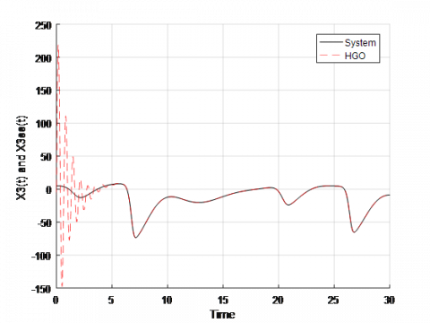
The results obtained by the application of the method of estimation by High Gain Observer are illustrated in Figure 12, 13 and 14. Indeed, we find a good behaviour because estimated and true values of the Colpitts system states are practically identical. The results can be considered acceptable as they show fast convergence in all states and a respectable behaviour as well.
The simulation of this observer shows the effectiveness and robustness of this observer to estimate the nonmeasured state of the system.
Figure 12. The time evolution of x1(t)and x1est(t) using the high gain observer
Figure 13. The time evolution of x2(t) and x2est(t) using the High gain observer
Figure 14. The time evolution of x3(t) and x3est(t) using the High gain observer
In the next section we will treat the sliding mode observer in order to compare the found results and test the effectiveness of the high gain observer.
After having used the high gain observer, we are interested in this section in the application of the sliding-mode observer in the case of the studied chaotic system. In order to find a Sliding Mode Observer (SMO) of the Colpitts circuit (5), the expression of $K\left(\tilde{x}^{1}\right)$ is given as follows:
$K\left(\tilde{x}^{1}(t)\right)=\eta C^{T} \operatorname{Csign}\left(\tilde{x}^{1}\right)$ (16)
with η>0 is real positive number and the "sign" is the sign function:
$\operatorname{sign}\left(\tilde{x}^{1}\right)=\left[\operatorname{sign}\left(\tilde{x}_{1}^{1}\right) \quad \cdots \quad \operatorname{sign}\left(\tilde{x}_{p}^{1}\right)\right]^{T}, : \tilde{x}_{i}^{1} \in R$
The sign function has a discontinuity that influences stability. To overcome these difficulties, continuous functions that have properties similar to those of the sign function must be used. This approach is widely used during the implementation of the sliding mode observer. Indeed, we use:
$K(\tilde{x})=\eta C^{T} C \operatorname{Tanh}(\tilde{x})$ (17)
where Tanh(.) designates the hyperbolic tangent function.
Finally, the sliding-mode observer for classes of non-linear systems (5) can be written in the following form:
$\dot{\hat{x}}=f(u, \hat{x})-\theta \Delta_{\theta}^{-1} S^{-1} \eta C^{T} \operatorname{CTanh}(\hat{x}(t)-x(t))$ (18)
So the equation (11) is rewritten:
$\dot{\hat{x}}=f(u, \hat{x})+\eta\left(\begin{array}{c}{3 \theta} \\ {3 \theta^{2}} \\ {\theta^{3}}\end{array}\right) \cdot \operatorname{Tanh}(\hat{x}-x)$ (19)
The equation system of the sliding mode estimator is therefore:
$\left\{\begin{array}{l}{\dot{\hat{x}}_{1}=-c \hat{x}_{3}-c \hat{x}_{2}-d \hat{x}_{1}+3 \eta \theta \cdot \operatorname{Tanh}\left(x_{1}-\hat{x}_{2}\right)} \\ {\dot{\hat{x}}_{2}=b \hat{x}_{1}+3 \eta \theta^{2} \cdot \operatorname{Tanh}\left(x_{2}-\hat{x}_{2}\right)} \\ {\dot{\hat{x}}_{3}=a \hat{x}_{1}-a \exp \left(-\hat{x}_{2}\right)+a+\eta \theta^{2} \cdot \operatorname{Tanh}\left(x_{3}-\hat{x}_{2}\right)}\end{array}\right.$ (20)
as given in the previous section $x_{1}=\frac{\dot{y}}{b} \cdot \operatorname{and} \cdot x_{3}=-\frac{1}{c}\left[\frac{1}{b} \ddot{y}+\frac{d}{b} \dot{y}+c y\right]$, so the system can be rewritten as follows
$\left\{\begin{array}{l}{\dot{\hat{x}}_{1}=-c \hat{x}_{3}-c \hat{x}_{2}-d \hat{x}_{1}+\frac{3}{b} \theta^{2} \eta \operatorname{Tanh}\left(x_{1}-\hat{x}_{2}\right)} \\ {\dot{\hat{x}}_{2}=b \hat{x}_{1}+3 \theta \eta \operatorname{Tanh}\left(x_{2}-\hat{x}_{2}\right)} \\ {\dot{\hat{x}}_{3}=a \hat{x}_{1}-a \exp \left(-\hat{x}_{2}\right)+a+\left(\frac{\theta^{3}}{b c}-\frac{3 d}{b c} \theta^{2}-3 \theta\right) \eta \operatorname{Tanh}\left(x_{3}-\hat{x}_{2}\right)}\end{array}\right.$ (21)
For the simulation, η=1 and the same initial conditions are used. Figure 15 shows the 3-D phase portrait of the Colpitts chaotic system (21) using the sliding mode observer.
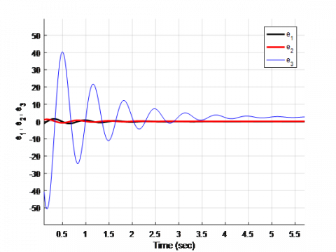
The Figure 16 illustrate the time evolution of the estimation error e1, e2 and e3 using the sliding mode observer.
Figure 15. 3-D sliding mode observer of chaotic Colpitts circuit
Figure 16. The time evolution of the estimation errors
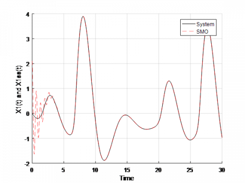
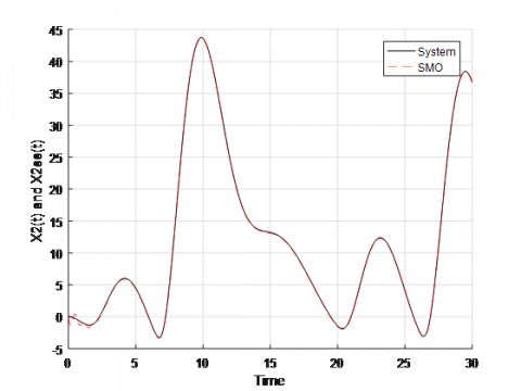
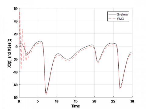
The results obtained by the Sliding Mode Observer are illustrated in Figure 17, 18 and 19.
Indeed, we find a good result since the estimated states and the states of the Colpitts system are the same. The results show fast convergence in all states and a respectable behavior as well.
These simulations show the effectiveness and the robustness of this observer to estimate the nonmeasured state of the system.
Figure 17. The time evolution of x1(t) and x1est(t) using the sliding mode observer
Figure 18. The time evolution of x2(t) and x2est(t) using the sliding mode observer
Figure 19. The time evolution of x3(t) and x3est(t) using the sliding mode observer
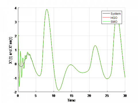
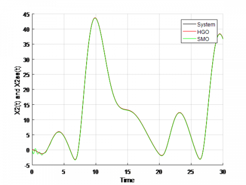
Figures 20, 21 and 22 present the high gain observer and the sliding mode observer in estimation of the Colpitts circuit. From these figures, we find a good corresponding betwwen the HGO and the SMO.
Figure 20. The estimation of x1(t) by the HGO and the SMO
Figure 21. The estimation of x2(t) by the HGO and the SMO
Figure 22. The estimation of x3(t) by the HGO and the SMO
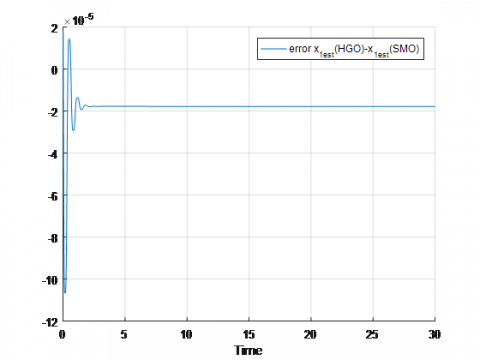
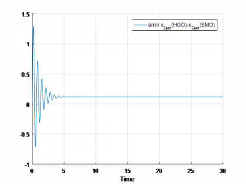
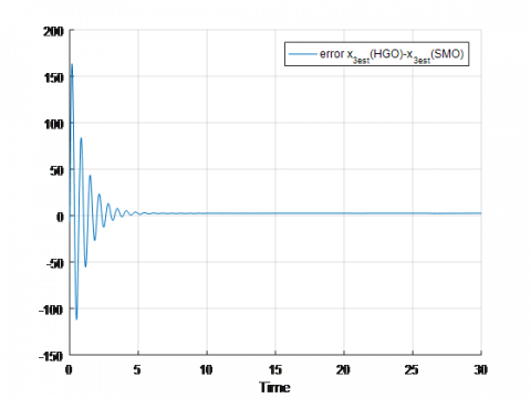
Figure 23. The error between the HGO and the SMO
Figure 24. The error between the HGO and the SMO
Figure 25. The error between the HGO and the SMO
Figures 23, 24 and 25 present the error, $e_{1}=\hat{x}_{1(H G O)}-\hat{x}_{1(S M O)}, e_{2}=\hat{x}_{2(H G O)}-\hat{x}_{2(S M O)}$ and $e_{3}=\hat{x}_{3(H G O)}-\hat{x}_{3(S M O)}$ between high gain observer and the sliding mode observer.
The MSE performance criteria is used to compare observers, as shown, in the table below.
Table 1. A comparative study between the approaches
|
State System |
MSE(HGO) |
MSE(SMO) |
|
x1(t) |
0.0520 |
0.0520 |
|
x2(t) |
0.0148 |
0.0302 |
|
x3(t) |
0.0311 |
0.0473 |
Comparing with the results obtained by these observers, the high gain observer showed a good ability to reconstruct the states of the chaotic system and providing a small mean squared compared to that of the sliding mode observer. Effectiveness of the high gain observer.
In this paper, we have proposed a high-gain observer and a sliding mode observer for the Colpitts system estimation. The synthesis of these observers took place under certain sufficient conditions arising directly necessary and sufficient conditions established for nonlinear systems. In this paper, the high gain observer gives good results. In future, a control method based on sliding mode observer will be developed.
[1] Kennedy, M.P. (1993). Three steps to Chao-Part II: A Chua's circuit primer. IEEE Trans. Circuits and Systems, 40(10): 657-674. https://doi.org/10.1109/81.246141
[2] Kennedy, M.P. (1994). Chaos in the Colpitts oscillator. IEEE Trans. Circuits and Systems, 41: 771-774. https://doi.org/10.1109/81.331536
[3] Kennedy, M.P. (1995). On the relationship between the chaotic Colpitts oscillator and Chua’s oscillator. IEEE Trans. Circuits and Systems, 42: 376-379. https://doi.org/10.1109/81.390276
[4] Pecora, L.M., Caroll, T.L. (1990). Synchronization in chaotic systems. Phy. Rev. Lett., 64(8): 821-824. https://doi.org/10.1063/1.4917383
[5] Gao, X.J., Hu, H.P. (2015). Adaptive-impulsive synchronization and parameter estimation of chaotic systems with unknown parameters bu using discontinuous drive signals. Appl. Math. Model, 39: 3980-3989. https://doi.org/10.1016/j.apm.2014.12.028
[6] Ma, J., Li, F., Huang, L., Jin, W.Y. (2011). Complete synchronization, phase synchronization and parameters estimation in a realistic chaotic system. Communications in Nonlinear Science and Numerical Simulation, 16(9): 3770-3785. http://dx.doi.org/10.1016/j.cnsns.2010.12.030
[7] Banerjee, S., Chowdhury, A.R. (2009). Lyapunov function, parameter estimation, synchronization and chaotic cryptography. Communications in Nonlinear Science and Numerical Simulation, 14(5): 2248-2254. http://dx.doi.org/10.1016/j.cnsns.2008.06.006
[8] Zhao, L.D., Hu, J.B., Fang, J.A., Cui, W.X., Xu, Y.L., Wang, X. (2013). Adaptive synchronization and parameter identification of chaotic system with unknown parameters and mixed delays based on a special matrix structure. ISA Trans., 52: 738. https://doi.org/10.1016/j.isatra.2013.07.001
[9] Zhu, F.L. (2009). Observer-based synchronization of uncertain chaotic system and its application to secure communications. Chaos, Solitons & Fractals, 40(5): 2384-2391. https://doi.org/10.1016/j.chaos.2007.10.052
[10] Jiang, X., Yang, J.Q., Zhu, F.L., Xu, L.Y. (2014). Observer-based synchronization of chaotic systems with both parameter uncertainties and channel noise. International Journal of Bifurcation and Chaos, 24(07). http://dx.doi.org/10.1142/S0218127414500953
[11] Alexander, L.F., Boris, A., Robin, J.E. (2008). Adaptive observer-based synchronization of chaotic systems with first-order coder in the presence of information constraints. IEEE Transactions on Circuits and Systems, 55(6). http://dx.doi.org/10.1109/TCSI.2008.916410
[12] Sharma, B.B., Kar, I.N. (2011). Eigenvalue analysis based control scheme for interconnected autonomous systems. TENCON 2011-2011 IEEE Region 10 Conference. http://dx.doi.org/10.1109/TENCON.2011.6129275
[13] Liao T.L., Tsai, S.H. (2000). Adaptive synchronization of chaotic systems and its application to secure communications. Chaos, Solitons and Fractals, 11(9): 1387-1396. https://doi.org/10.1016/S0960-0779(99)00051-X
[14] Dimitriev, A., Panas, A., Starkov, S. (2001). Direct chaotic communications in microwave band, in Proc. European Conf. on Circuit Theory and Design, Espoo, Finland, Aug.
[15] Tamaševičius, A., Čenys, A., Mykolaitis, G., Namajūnas, A. (1998). Synchronization of chaos and its application to secure communication. Lithuanian Journal of Physics, 38(1): 33-37.
[16] Maximov, N., Panas, A., Starkov, S. (2001). Chaotic oscillators design with preassigned spectral characteristics, in Proc. European Conf. on Circuit Theory and Design, (Espoo, Finland), pp. 429-432.
[17] Farza, M., M'Saad, M., Rossignol, L. (2004). Observer design for a class of MIMO nonlinear systems. Automatica, 40: 135-143. http://dx.doi.org/10.1016/j.automatica.2003.08.008
[18] Martinez-Guerra, R., Pérez-Pinacho, C.A., Gomez-Cortés, G.C., Cruz-Victoria, J.C., Mata-Machuca, J.L. (2014). Experimental synchronization by means of observers. Journal of Applied Research and Technology, 12: 52-62.
[19] Mkaouar, H., Boubaker, O. (2017). Robust control of a class of chaotic and hyperchaotic driven systems. Pramana – J. Phys. 88-90. http://dx.doi.org/10.1007/s12043-016-1316-5
[20] Khalifa, N., Filali, R.L., Benrejeb, M. (2016). A fast selective image encryption using discrete wavelet transform and chaotic systems synchronization, Information technology and control, 45(3): 235-242. http://dx.doi.org/10.5755/j01.itc.45.3.12650
[21] Gang, X., Jing L, Liwen W. (2018). Containerized microservices: Structures and dynamics. Advances in Modelling and Analysis A. 55(1): 1-10. https://dx.doi.org/10.18280/ama_a.550101
[22] Abdulganiy, R.I., Akinfenwa, O.A., Okunuga, S.A., Oladimeji, G.O. (2017). A robust block hybrid trigonometric method for the numerical integration of oscillatory second order nonlinear initial value problems. AMSE JOURNALS-AMSE IIETA publication-2017-Series: Advances A, 54(4): 497-518. https://dx.doi.org/10.18280/ama_a.540404