© 2018 IIETA. This article is published by IIETA and is licensed under the CC BY 4.0 license (http://creativecommons.org/licenses/by/4.0/).
OPEN ACCESS
This paper attempts to solve the problem of material selection for resonance panels in Chinese musical instruments, which are mostly made of wood. For this purpose, the author combined the Gaussian mixture model (GMM) and support vector machine (SVM) into a classification and recognition algorithm of wood vibration signals, and adopted the approach to classify and recognize resonance panels of different Chinese musical instruments. The application results show that our method achieved a recognition rate greater than 90%, outperformed the strategy of using the GMM as the only classifier, and overcame the decline of recognition rate of the SVM facing a huge amount of data. The research findings shed new light on the material selection and quality improvement of Chinese musical instruments.
gaussian mixture model (GMM), gabor, chinese musical instruments, support vector machine (SVM)
As the carrier of traditional culture, China’s national musical instrument has a long history of development (Luo and Tang, 2013). It records the glorious music culture of China and the outstanding wisdom and creativity of its ancestors. Wood is an indispensable raw material for making musical instruments. Wood, like other elastic materials, can generate and propagate vibrations under the action of impact force or periodic external force. This reaction to external force vibration is the source of sound effects produced by wood. The vibrating wood surface will excite the surrounding air and use air as the medium to transmit vibrations into the human ear in the form of waves. The wood with good acoustic property has excellent acoustic resonance and vibration spectrum characteristics, and it can give a beautiful sound by radiating the sound energy from its own vibration under the action of the impact force. Therefore, the study of the wood vibration sound signal characteristics is of great significance for the manufacture of musical instruments. The studies for the wood vibration characteristics by domestic and foreign experts and scholars (Shen et al., 2002; Chen, 1988; Ono and Norimoto, 1983) can be broadly divided into several aspects, such as vibration characteristics method, the interrelationship between vibration parameters, the selection of musical instrument soundboards, and the analysis of characteristics etc.
The features used in the field of voice recognition are mostly divided into the following categories, such as short-term energy, zero-crossing rate, Mel-Frequency Cepstral Coefficients (MFCC) (Bhalke et al., 2016), Spectral Centroid, Sub-band Energy, Perceptual Linear Prediction (PLP), LPCC (Ai et al., 2006), and Gabor (Wang et al., 2014), or a combination of these features. Currently the commonly used sound classification algorithms are GMM, SVM (Jung and Yong, 2017), KNN (Wang et al., 2006), END, Bayes, and HMM (Brognaux and Drugman, 2016) etc. In the mid-1970s, the voice recognition of Hidden Markov model (HMM) based on DTW and statistical methods appeared. HMM can effectively describe the time-varying characteristics of speech signals and solve the problems encountered by DTW in computing and segmenting continuous sound primitives. The literature (Radhakrishnan and Divakaran, 2005) proposed an audio monitoring system applied to the railway environment, where the MFCC feature is used to train the GMM classifier and recognize screams and gunshots. KNN is widely used in various fields for its simple realization and high classification accuracy. Its drawback is that it requires a large storage overhead and the boundary classification error is large. END is also a classification algorithm with the higher classification accuracy. However, due to the high complexity of the END calculation time, it is difficult to implement the classification problem with many data types and large data volumes. SVM is a new type of machine learning method developed on the basis of statistical learning theory (Vapnik, 1997). It solves practical problems such as non-linearity, small sample size and high dimensionality, and has become one of the research hotspots in machine learning; it has also successfully applied to classification, time series prediction and function approximation, etc., so as to reflect the differences between categories to a greater extent in terms of classification.
This paper intends to introduce related methods of sound recognition into the study so as to explore new ideas and methods. In view of the many advantages of the SVM method, this paper proposes one method based on the combination of different sound eigenvalues to establish a hybrid model of GMM and SVM and classify the vibration sound signals of wood. Then it extracts three features of LPCC, MFCC and Gabor for comparison experiments. This paper proves the feasibility and correctness of the GMM-SVM model to classify the sound signals of wood vibration.
The rest of the paper is organized as follows. In Sect. 2, highlights the process of feature extraction of wood sound. Then the GMM model and SVM classifier and an overall about algorithm design will be described in Sect. 3. The test results are presented and discussed in Sect. 4. Finally, Sect. 5 concludes the paper and describes the future work.
The basic task of feature extraction is to analyze and process the preprocessed sound signal and extract the important and useful information for sound recognition. The selection of feature parameters is one key issue for sound classification and the quality of feature parameters directly affects the classification accuracy. Therefore, the feature parameters that can reflect the important characteristics of wood vibration sound should be extracted firstly, and then the data can be given to the classifier for training and classification recognition. This paper selects three commonly used sound features: LPCC, MFCC and Gabor.
2.1. LPCC feature
The Linear Prediction Coefficient (Jiang and Zhang, 2009) (LPC) technique is the theoretical and calculation basis for solving the Linear Prediction Cepstral Coefficient (LPCC). To ensure the stability of sound feature parameters and the effect of sound recognition, LPC isn’t generally used as the feature parameter of sound signal in sound recognition systems, but it is subjected to homomorphic signal processing to obtain the LPC cepstral coefficient. The LPCC is recursively derived from linear prediction coefficients. The iterative relationship is given as:
$\begin{aligned} c_{0} &=\log G^{2} \\ c_{m} &=a_{m}+\sum_{k=1}^{m-1} \frac{k}{m} c_{k} a_{m-k}, 1 \leq m \leq p \\ c_{m} &=\sum_{k=1}^{m-1} \frac{k}{m} c_{k} a_{m-k}, m>p \end{aligned}$ (1)
When the order of LPCC is smaller than that of LPC, the second equation in formula (1) is used. When the order of LPCC is greater than the that of LPC, the third equation is used.
2.2. MFCC feature
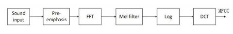
MFCC is the feature that utilizes the human ear’s different perception of different frequency signals. A non-linear Mel frequency scale is used to simulate the auditory system of the human ear by combing the human ear’s auditory perception characteristics with the sound production mechanism. It can be widely used in all areas of sound signal processing.
The extraction process of MFCC feature parameter is shown in Figure 1:
Figure 1. Extraction process of MFCC parameter
In the actual operation process, the specific solving process of MFCC feature parameters is given as follows:
(1) The wood vibration sound signal is divided into a series of consecutive frames. Then the Hamming window framing is added, where each frame contains N=512 samples, and the adjacent frame has 256 samples overlapping. Let the sound signal time domain signal be x(n), the i-th frame sound signal xi(n) can be expressed as:
$x_{i}(n)=x(i \times N+n) \omega(n), 0 \leq n \leq N-1$ (2)
where, $\omega(n)$ is Hamming window,
$\omega(n)=\left\{\begin{array}{cc}{0.54-0.46 \cos \left(\frac{2 \pi n}{N-1}\right), 0} & { \leq n \leq N-1} \\ {0} & {, \text { other }}\end{array}\right.$ (3)
(2) The signal is converted from the linear frequency to the Mel frequency scale. The conversion formula is expressed as
$\operatorname{Mel}(f)=2595 \lg \left(1+\frac{f}{700}\right)$ (4)
(3) The triangular filter bank is configured on the Mel frequency axis, and the center frequency c(l) of each triangular filter is uniformly spaced. The corresponding upper and lower limit frequencies can be represented by h(l) and o(l), respectively. The cutoff frequency of the signal determines the number of filters L. Therefore, the upper limit, center and lower limit frequencies between adjacent triangular filters have the following relationship:
$c(l)=h(l-1)=\circ(l+1)$ (5)
(4) One logarithmic transformation on the output of the filter is performed. This shall not only compress the dynamic range of the signal, but also convert the convolutional relationship into a linear relationship by the homomorphic transformation so as to separate the noise.
(5) Finally, the discrete cosine transform on the logarithmic spectrum is made to remove the correlation of the spectrum, map the signal to the low-dimensional space, and obtain MFCC. The discrete cosine transform is expressed as:
$C_{n f c c}(j)=\sqrt{\frac{2}{N}} \sum_{l=1}^{L} \log m(l) \cos \left\{\left[l-\frac{1}{2}\right] \frac{j \pi}{L}\right\} 0 \leq i \leq \mathrm{D}$ (6)
where L is the number of Mel filters and D is the dimension of the MFCC feature.
2.3. Gabor feature
The Gabor filter bank consists of a set of two-dimensional Gabor filters, where each filter is defined by the time-frequency domain envelope function and the time-frequency carrier function. The Gabor filter function is defined as:
$g\left(k_{0}, n_{0}, \omega_{,}, \omega_{n}, k, n, v_{k}, v_{n}, \varnothing\right)$
$=s_{a_{k}}\left(k-k_{0}\right) s_{\omega_{n}}\left(n-n_{0}\right) \cdot \frac{h_{V_{k}}}{2 \alpha_{k}}\left(k-k_{0}\right) h_{\frac{v_{n}}{2 \omega_{n}}}\left(n-n_{0}\right) \cdot e^{i \otimes}$ (7)
where k is the frequency index, n is the frame index, k0 is the carrier frequency, n0 is the center of the time frame, ωk is the spectrum modulation frequency, ωn is the time modulation frequency, vkand vn are the half-cycle number of the carrier in the frequency and time domain dimensions respectively, and ∅ is an additive global phase.
The Gabor feature is a time-frequency feature whose extraction process is shown in Figure 2:
Figure 2. Extraction process of gabor parameter
First, the sound signal y(n) is windowed and pre-emphasized, using Hamming window. Then, the discrete Fourier transform is applied to the sound signal for transforming the signal into the frequency domain Yl,k, and the log spectrum of the signal is logarithmically transformed by Mel spectrum $\hat{Y}_{l, m}$:
$Y_{l, k}=\sum_{n=0}^{N-1} y\left(n+l \cdot n_{s}\right) \omega(n) \mathrm{e}^{-j 2 \pi k n / N} \quad 0 \leq k \leq N-1$ (8)
$\hat{Y}_{l, m}=\log \left(\sum_{k=0}^{N-1}\left|Y_{l, \mathbf{k}}\right| \cdot F_{k, m}\right) \quad 0 \leq m \leq M-1$ (9)
where N is the window length, ns is the sampling frequency, and M is the number of MEL filter. Then, the logarithm Mel spectrum coefficient Y is sent to the two-dimensional Gabor filter, and the real part of the Gabor filter output is taken as the Gabor feature of the signal, as shown in formula (10):
$\mathrm{G}_{n, k}\left(k_{0}, n_{0}, \omega_{k}, \omega_{n}, v_{k}, v_{n}\right)$
$=\Re\left\{\sum_{\mu, \lambda} \hat{Y}_{\mu, \lambda} g\left(\mu+k, \lambda+n ; k_{0}, n_{0}, \omega_{k}, \omega_{n}, v_{k}, v_{n}\right)\right\}$ (10)
When one Gabor filter bank is applied to each Mel filter, a high-dimensional feature representation shall be obtained correspondingly, e.g., in this paper, 23 Mel filters and 41 Gabor filters are used, so Gabor filter output has 23*41=943 dimensions. The literature (Schädler et al., 2012) indicated that the filter output of the adjacent channel is highly correlated, thus, the output of the Gabor filter can be reduced dimensionally.
3.1. GMM model classifier
At present, GMM as a commonly used classifier has been used in many fields of sound signal processing, and especially it has achieved good results in the field of audio retrieval and audio event detection. The GMM model describes the statistical distribution of features through the linear weighting of the Gaussian probability density function. The spatial distribution of feature parameters determines the model parameter values. One M-order GMM is a weighted sum of M Gaussian probability density functions, as shown in Formula (11):
$P(\mathbf{a} | \lambda)=\sum_{i=1}^{M} P_{i} b_{i}(\mathbf{a})$ (11)
where, a is a D-dimensional feature vector; bi(a) is the D-dimensional Gaussian distribution function that represents a Gaussian mixture model component; Pi is the weighting factor of the corresponding component bi(a). For bi(a) and Pi, it can be expressed as:
$b_{i}(\mathbf{a})=\frac{1}{(2 \pi)^{D_{2}}\left|\vec{\Sigma}_{i}\right|^{1 / 2}} \exp \left\{-\frac{1}{2}\left(\mathbf{a}-\mu_{i}\right) \vec{\Sigma}_{i}^{-1}\left(\mathbf{a}-\mu_{i}\right)\right\}$ (12)
$\sum_{i=1}^{M} \omega_{i}=1$ (13)
where, μi is the mean vector; $\vec{\Sigma}_{i}$ is the covariance matrix. Therefore, the GMM consists of the parameter mean vector, the covariance matrix, and the mixing weights. It is expressed as:
$\lambda=\left\{\omega_{i}, \mu_{i}, \vec{\Sigma}_{i}\right\} \quad \mathrm{i}=1, \cdots, M$ (14)
3.1.1. GMM EM algorithm of GMM
The GMM parameters represents the individual characteristics of the wood board vibration signal Therefore, a set of parameters that determine the probability distribution should be found during the identification in order to maximize the probability of representing the sound characteristics of the wood board vibration. Usually, the EM algorithm is used to achieve the maximum likelihood estimation. By iteratively estimating the parameters of the GMM by the EM algorithm, when the value of the likelihood function reaches its maximum, the iteration stops. The EM algorithm parameters are estimated in the following procedures:
(1) Calculate the unknown z (each classification) using the parameters obtained in Step M, to obtain the conditional distribution of the observed data,
$P(z | y, \theta)=\frac{p(y, z | \theta)}{p(y | \theta)}=\frac{p(y | z, \theta) p(z | \theta)}{\sum(p | z, \theta) p(z | \theta)}$ (15)
where, P(z|y,θ) is the likelihood function of complete data, p is the joint probability density function of the complete data; (y, z) is the sample set, y is the observation data, z is the missing data, P(z|y,θ) is the conditional probability of missing data, and P(z|θ)is the distribution of missing data.
(2) Calculate new mean, variance, and weight;
$\mu_{i}=\frac{\sum_{j=1}^{m} p\left(z_{j}=i | y_{j}, \theta_{t}\right) y_{j}}{\sum_{j=1}^{m} p\left(z_{j}=i | y_{j}, \theta_{t}\right)}$ (16)
$\sigma_{i}=\frac{\sum_{j=1}^{m} p\left(z_{j}=i | y_{j}, \theta_{t}\right)\left(y_{j}-\mu_{j}\right)\left(y_{j}-\mu_{j}\right)^{T}}{\sum_{j=1}^{m} p\left(z_{j}=i | y_{j}, \theta_{t}\right)}$ (17)
$p\left(z_{j}=i | \theta\right)=\frac{\sum_{j=1}^{m} p\left(z_{j}=i | y_{j}, \theta_{t}\right)}{\sum_{k=1}^{n} \sum_{j=1}^{m} p\left(z_{j}=k | y_{j}, \theta_{t}\right)}$ (18)
(3) Substitute μj,σj,p(zj=i|θ) into step (15) to recalculate until the sample set no longer significantly changes the likelihood function of each classification.
When training the GMM by the EM algorithm, it is necessary to first determine the order M of and the initial parameters of the model: weight, mean, and variance. The clustering method is generally adopted for the selection of initial parameters. There are many clustering algorithms, such as K-means algorithm, STING algorithm, CLIQUE algorithm etc. The K-means algorithm, by centralized division of the complete data set and incomplete searching, can ensure the maximum of the given objective function value maximum under certain criteria. It has the characteristics of theoretical reliability, fast convergence, and efficient processing of large data sets. Therefore, K-means algorithm is selected in this paper.
In the training phase, the model is created for each wood vibration signal, i.e., the sound feature vectors are first clustered to obtain the initial values of the weights, the mean and the covariance matrix, and then a set of parameters is determined for each wood by iteration according to the EM algorithm, which are used as model parameters. Through the K-means algorithm, the EM algorithm obtains the relatively theoretical and stable initial value. The K-means algorithm is the key initialization step in the EM algorithm and a very widely used clustering method.
3.2. SVM classifier
SVM was proposed by Vapnik (1999). It has particular advantages in solving small-sample, non-linear and high-dimensional data pattern recognition. Given a set of training samples, each of which is marked as one of two categories, the SVM can construct a non-probabilistic binary linear classifier model so that a new sample can be classified into its category. The principle of SVM is to map the points in the low-dimensional space to the high-dimensional space, so that these data can be linearly separable in the high-dimensional space, and then use the linear partition principle to divide the category boundaries. The main idea of SVM is to establish a hyperplane as the decision surface, which maximizes the interval between samples to be divided, and realizes the transformation from the classification problem into a constrained min/max problem, as shown in the following:
$\min \frac{\|\omega\|^{2}}{2}+C \sum_{I=1}^{N} \zeta_{i} \quad \mathrm{C}>0$
s.t $\quad \mathrm{y}_{i}[(\omega \mathrm{x})+b] \geq 1-\zeta_{i} \zeta_{i}>0$
$\forall i=1,2, \cdots, N$ (19)
where: ζi is slack variable; C is the penalty factor, and N is the number of samples.
In formula (19), it can be seen that those influencing the SVM model accuracy are slack variable ζ and penalty factor C. The slack variable ζ ensures the SVM to have fault tolerance when the sample is regressed, while the penalty factor C is to solve the problem that the SVM classifier makes the target ‖w‖ smaller for a small number of discrete points. The kernel function (ωx) reflects the degree of correlation of each support vector and realizes the transformation of model solution into a planning problem with constraint by mapping the inseparability between the vector and x in the low-dimension space to the high-dimensional space and then making the inner product. To select the kernel functions and determine the kernel function parameters are key points and difficulties. The commonly used kernel functions are shown in Table 1.
Table 1. Common kernel function
|
Kernel function name |
Kernel function expression |
|
Linear Kernel |
$k\left(\mathrm{x}_{i}, \mathrm{x}_{j}\right)=\mathrm{x}_{i}^{T} x_{j}+c$ |
|
Polynomial Kernel |
$k\left(\mathrm{x}_{i}, \mathrm{x}_{j}\right)=\left(\alpha x_{i}^{T} \mathrm{x}_{j}+\mathrm{c}\right)^{d}$ |
|
RBF Kernel |
$k\left(\mathrm{x}_{i}, \mathrm{x}_{j}\right)=\exp \left(-\alpha\left\|\mathrm{x}_{i}-\mathrm{x}_{j}\right\|^{2}\right)$ |
|
Sigmoid Kernel |
$k\left(\mathrm{x}_{i}, \mathrm{x}_{j}\right)=\tanh \left(\alpha\left(\mathrm{x}_{i}^{T} \cdot \mathrm{x}_{j}\right)+\mathrm{c}\right)$ |
Recognition of wood vibration signals is a multi-class classification issue. The single 2-class SVM classifier cannot solve this issue. There are generally two kinds of treatment methods, namely, one-to-many method and one-to-one method. In this paper, the one-to-many method was adopted to train and identify samples, and to extend the 2-class classification problem to multiple classes; this method can easily classify each optimization problem at fast speed of classification. If there are N different wood vibration signals in this method, the nth is defined as +1 class, and the others are combined as -1 class, thus, a two-class classifier is obtained. In this way, N classifiers can be finally obtained. In the recognition process, the sounds to be tested are input into N classifiers, and the decision function values are calculated by formula (20) and (21).
SVM classifier is expressed as:
$f_{n}(x), n=1,2, \cdots, N$ (20)
Decision function is given as:
$f(x)=\arg \max \left\{f_{1}(x), \cdots f_{N}(x)\right\}$ (21)
3.3. GMM-SVM classifier
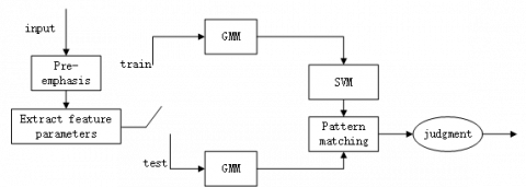
Studies have shown that GMM and SVM have very different recognition rates on the same training data, indicating that they are complementary in some aspects. Therefore, if the wood vibration signal recognition system can integrate the advantages of both models, the recognition rate will be improved to some extent. In practical applications, the SVM training algorithm is complex and requires a large amount of calculations, making it difficult to process large amounts of sample data. The hybrid model combining the advantages of GMM and SVM together, can effectively solve the problems of SVM training algorithm above. In this paper, the wood vibration signal recognition system is established by GMM-SVM method. Based on the eigenvectors calculated by the GMM, the SVM is used to perform the optimal classification, establish the sample database, and complete the training process. Besides, in the recognition process, the decision function is used to discriminate the sound samples of wood vibration. Fig.3 depicts the structure of wood vibration. signal recognition system based on GMM-SVM.
Figure 3. Wood vibration signal recognition system structure based on GMM-SVM
The recognition process is made are as follows:
(1) After preprocessing the training sounds, extract the feature parameters, and then make GMM training by EM algorithm to to obtain the mean parameters. If there are N woods, the mean values are μ1, μ2,..., μn respectively.
(2) Using the one-to-many method to train the SVM model; calculate the distance $d_{n m}^{1}, \mathrm{d}_{r n n}^{2}, \cdots, \mathrm{d}_{n m}^{N}$ from each sound signal to the m-th mean value parameter of the n-th wood vibration sound signal, and finally obtain an N-dimensional training sample $d_{n m}^{1}, \mathrm{d}_{r n n}^{2}, \cdots, \mathrm{d}_{n m}^{N}$.
(3) Repeat step (2) to obtain all SVM training samples and finally achieve the N SVM recognition models.
(4) For the sound sample to be tested, take the similar method as step (1) to obtain the final test sample.
(5) Compare the test sample with each SVM model. According to the classification criteria, the wood level corresponding to the maximum output value is the recognition result.
4.1. Data collection
The professional recording pen was used in the quiet laboratory environment with relatively little noise. The experimental materials were 30 wood boards of paulownia elongata of the same size and 3 different quality grades. There were 10 boards per quality grade; for each board took, 30 fixed positions were taken and recorded for 60s respectively, to obtain the mono sound file at sampling rate 32 kHz. In order to reduce the complexity of voice data, 8 kHz sampling rate was adopted for re-sampling, i.e., down-sampling, and then the voice file was saved as a sound file with a quantization number of 16-bit, wav format, followed by preprocessing.
4.2. Preprocessing
CoolEdit software was used to remove noise from the original sound sample, and then the high-pass filter as adopted to eliminate the low-frequency noise in the audio, because there existed non-voice segments in the recorded sound data. High-pass filter conversion function is H(z)=1-kZ-1, where parameters k is set to be 0.9375. After the signal passed through the high-pass filter, the signal that was originally only floating in the low-frequency part was adjusted to make it sound clearer. All sound files were intercepted into about 2s data for training and testing. Sound signal before and after noise removal is shown as follows:
Figure 4. Waveform of original wood vibration sound signal
Figure 5. Waveforms of wood vibration sound signal after denoising
4.3. Experimental results discussion
Through experiments, the selection of the mixing degree M of the GMM, the recognition effect of different sound features, and the recognition effect of different classifiers were studied. The recognition rates of GMM system and GMM-SVM system based on MFCC features at different mixing degree are shown in Table 2.
Table 2. Recognition rates of GMM and GMM-SVM at different mixing degrees
|
mixing degree |
GMM recognition rate% |
GMM-SVM recognition rate% |
|
8 16 32 64 |
79.1 85.4 88.6 86.2 |
81.4 89.1 90.9 91.0 |
In Table 2, it can be seen that the recognition rate of GMM system and GMM-SVM system increase with the mixing degree, and when the mixing degree is the same, the recognition rate of GMM-SVM system is always higher than that of GMM system. At the mixing degree 8, 16, and 32, the recognition rate of both increases rapidly, but when the mixing degree is more than 32, the recognition rate of the GMM system almost no longer increases, despite the increase of the mixing degree, whereas the recognition rate of GMM-SVM system is still slowly increasing. Therefore, the mixing degree M has a great influence on the recognition rate of the system. When M is small, GMM cannot describe the acoustic characteristics of wood well, and then the classification result of SVM is not accurate enough, so as to decrease the recognition rate of the system. When M is too high, the training of GMM takes too much time, and SVM training is also faced with large sample problems, leading to the reduced system identification performance. Thus, the moderate mixing degree M of the GMM model should be selected, by taking 32 in this paper. A process of extracting LPCC and MFCC features, the frame length was 512 points and the frame shift were 256 points. The LPCC feature of each frame took 12-dimensions, and its first-order differential dynamic features were also taken, to obtain a total of 24 eigenvectors. The LPCC, MFCC and Gabor features characterize the cepstral domain and time-frequency domain of the sound event respectively, belonging to two different types of sound features. Besides, the Hamming window was used to extract the Gabor features, with 41 Gabor filters. Each Gabor filter was convolved with 23 log Mel frequency bandwidths in the frequency range from 64 Hz to 4000 Hz. The secondary sampling was made for Gabor filter output, and the initial feature of 41*23=943 dimension was reduced to 311 dimensions. Based on the experimental results in Table 2, the M value was chosen as 32 in this experiment. The experimental results of the 3 different sound features are shown in Table 3.
Table 3. Recognition rates of GMM and GMM-SVM under different sound features
|
feature |
GMM recognition rate% |
GMM-SVM recognition rate% |
|
LPCC MFCC Gabor |
78.3 88.6 89.8 |
81.6 90.9 91.9 |
In this paper, three different methods were used to extract feature parameters. Besides, the sound classification method combining GMM model with SVM classifier was adopted and compared with the GMM used alone as classifier. Finally, the experiments were performed at different mixing degrees. In the same environment, the experimental results show that the classification method based on GMM-SVM hybrid model has the characteristics of simple structure and high classification accuracy, and it can be practically applied in the wood vibration sound classification system. In future, more studies should be made by combing the GMM with other theories, in order to apply it more effectively to the field of wood vibration sound recognition.
This research is supported by the Fundamental Research Funds for the Central University (2572018BH03), The National Natural Science Found project (31670717).
Ai C., Zhao H., Ma R., Dong X. (2006). Pipeline damage and leak detection based on sound spectrum LPCC and HMM. International Conference on Intelligent Systems Design and Applications. IEEE, pp. 829-833. http://dx.doi.org/10.1109/ISDA.2006.215
Bhalke D. G., Rao C. B. R., Bormane D. S. (2016). Automatic musical instrument classification using fractional fourier transform based- MFCC features and counter propagation neural network. Journal of Intelligent Information Systems, Vol. 46, No. 3, pp. 425-446. https://doi.org/10.1007/s10844-015-0360-9
Brognaux S., Drugman T. (2016). HMM-based speech segmentation: Improvements of fully automatic approaches. IEEE Press.
Chen J. (1988). Preliminary study on musical instrument materials in Guangxi. Journal of Guangxi Agricultural College, No. 2, pp. 81-82.
Jiang B., Zhang J. (2009). Linear prediction coding and its application in G.729. Journal of Zhejiang University of Technology, Vol. 37, No. 2, pp. 196-200.
Jung S. H., Yong J. C. (2017). Performance comparison between GMM and SVM for scream sound detection. Next Generation Computer and Information Technology, pp. 146-149.
Luo J., Tang H. (2013). Inheritance and development of chinese folk instruments. Forward Position, Vol. 30, No. 7, pp. 166-167.
Ono T., Norimoto M. (1983). Study on Young's modulus and internal friction of wood in relation to the evaluation of wood for musical instruments. Limnology & Oceanography, Vol. 22, No. 4, pp. 611-614.
Radhakrishnan R., Divakaran A. (2005). Systematic acquisition of audio classes for elevator surveillance. Image and Video Communications and Processing, Vol. 5685, pp. 1-8. https://doi.org/10.1117/12.587814
Schädler M., Meyer B. T., Kollmeier B. (2012). Spectro-temporal modulation subspace-spanning filter bank features for robust automatic speech recognition. The Journal of the Acoustical Society of America, Vol. 131, No. 5, pp. 4134-4151. https://doi.org/10.1121/1.3699200
Shen J., Liu Y., Liu Z., Yu H. P., Gang Y. J., Hetian C. J. (2002). Effect of microfibril angle on vibration properties of picea wood. Journal of Northeast Forestry University, Vol. 30, No. 5, pp. 50-52. http://dx.chinadoi.cn/10.3969/j.issn.1000-5382.2002.05.015
Temko A., Nadeu C. (2006). Classification of acoustic events using SVM-based clustering schemes. Pattern Recognition, Vol. 39, No. 4, pp. 682-694. http://dx.doi.org/10.1016/j.patcog.2005.11.005
Vapnik V. N. (1997). The nature of statistical learning theory. IEEE Transactions on Neural Networks, Vol. 8, No. 6, pp. 1564. https://link.springer.com/book/10.1007%2F978-1-4757-2440-0
Vapnik V. N. (1999). An overview of statistical learning theory. IEEE Transactions on Neural Networks, Vol. 10, No. 10, pp. 988-999. https://doi.org/10.1109/72.788640
Wang J. C., Lin C. H., Chen B. W., Tsai M. K. (2014). Gabor-based nonuniform scale-frequency map for environmental sound classification in home automation. IEEE Transactions on Automation Science & Engineering, Vol. 11, No. 2, pp. 607-613. http://dx.doi.org/10.1109/TASE.2013.2285131
Wang J. C., Wang J. F., He K. W., Hsu C. (2006). Environmental sound classification using hybrid SVM/KNN classifier and MPEG-7 audio low-level descriptor. International Joint Conference on Neural Networks, pp. 1731-1735. http://dx.doi.org/10.1109/IJCNN.2006.246644