Detection and Cooperative Communications for Deployment Sensor Networks

Depending on the number of nodes of the network and the surface of the cover field, some nodes cannot directly transmit their messages to the collector node. Thus, the collaboration between the nodes to guarantee this transmission becomes a requirement. In this way, the messages are relayed by the intermediate nodes by establishing multi-jumping paths between a remote source and the well. This process of routing messages from a source node of the network to a recipient node is called routing. Thus, for a sensor network to be effective, the setting up of a routing algorithm becomes inevitable [3].

2.1 Routing concepts

There are two classes of routing protocols: distance vector routing and link state routing, so a routing protocol can be proactive or reactive [4].

2.1.1 Distance vector routing

This protocol class is based on an exchange between neighboring nodes and the node sending information about the list of destinations available to it and the corresponding cost. Routing protocols based on the most famous distance vector for ad hoc networks are: DSR, DSDV6, AODV and the new RPL protocol.

2.1.2 Link state routing

This protocol is known under the name of 'Shortest Path First'. This routing is based on the information collected and disseminated periodically on the state of the links in the network to update its description base describing a general view of the topology of the network. The main routing protocols in ad hoc networks that belong to this class are as follows: TORA, OLSR, etc.).

2.1.3 Proactive / reactive routing protocol

The proactive protocol builds its routing table before the request is made. A system of periodic exchange of control packets is put in place so that each node can build the network topology in a distributed fashion. The main proactive protocols are OLSR, FSR. On the other hand, a node using the reactive protocol completely ignores the topology of its network it updates its routing table only after having received a routing request from a neighboring node.

2.2 Detection in wireless sensor network

The trivial meaning of the term 'detection' is the process of capturing physical quantities related to environmental conditions (movement, temperature, humidity, light, etc.). The processing is based on the compatibility of the data captured by deploying different algorithms, either by comparing the previous state with the current state or using a consensus in order to eliminate the outliers and transmit a single common value to the sink.

2.2.1 Detection methods

1. Detection aggregation: based on statistical tests such as Maximum, Average [5] or a discretized classification of data [6] to aggregate the values captured over time;

2. Spatial and temporal correlation: Periklis et al. [7] list all the sensors in good condition and use them as references to test the other sensors. The simulation results show that this method consumes a lot of landfill and congestion. The use of cluster architecture is adopted to reduce this overhead [8];

3. Average consensus: The algorithms based on this principle conform to calculate the average between the recorded measurements and distribute it between neighboring sensors [9]; and

4. Consensus of beliefs: this consensus [10] is an algorithm derived from Bayes rule where a set of sensors try to harmonize on the most probable classification of an event.

2.2.2 Detection methods comparison

In Table 1, we present a classification of the protocols described in the previous section 2.1.

Table 1. Advantage and disadvantage of detection methods

2.3 Simulator Cooja

Contiki OS Java Simulator is a sensor network emulator that can house a compiled program in order to test a scenario before loading it into flash memory of real nodes as in the TI MSP430 platform (Figure 2).

2.png

Figure 2. Interface graphique Cooja

2.4 Routing protocol - RPL

The basic principles of the protocol are [11, 12]:

1. Routing: the path discovery is based on the quality of the signal, the density of nodes and active path is represented by its costs;

2. Route selection: a reliable route relies on signal strength (RSSI);

3. Road quality criteria: signal strength (RSSI), number of hops, available energy and error rate (outliers);

4. Changing the path: the path initially traced can be corrected later depending on the strength of the signal and the total number of nodes visited in the event of failure of the main road; and

5. Constraint-based routing: The life of a node depends on the battery and diversity of node types and their characteristics (memory, location, collector, etc.).

2.5 Signal Strength (RSSI)

Received Signal Strength Indication informs us by a measurement on the intensity of the received signal Rx. It is an essential parameter for radiolocation applications, due to its simplicity and low cost, but its accuracy can be degraded by noise caused by stable, moving objects and obstacles or by diffraction or refraction of radio waves [13].

$R S S I=-(10 * n * \log d+A)$            (1)

n: Constant - signal propagation.

d: distance between the transmitter Tx and the receiver Rx.

A: Signal strength received for 1 meter distance.

So the distance is calculated from the RSSI:

$d=10^{((A b s(R S S I)-A) 10 * n)}$            (2)

According to Eq. (1), if A increases then RSSI increases. Thus the relation between the power of the transmitted signal Tx and the distance of the signal traveled ″d″ is exponential; but in reality this relationship is only as implicit in theory.

In this article we focus on a well-chosen configuration to collect values by exploiting the received signal power (RSSI).

The proposed methods were tested by a simulation on the CONTIKI / COOJA platform. For our simulation the mote selected is TmoteSky is a wireless sensor board from Moteiv [16]. This is an MSP430 based board with an 802.15.4 compatible CC2420 radio chip, 1megabyte external serial flash memory and two light sensors. TmoteSky port was integrated into the Contiki building system in March 2007. The functionality of the MSP430 F1611 module is detailed in the Texas Instruments MSP430x1xx Series User Guide available in Ref. [17].

We place the sink node (called mote1) at a fixed initial position. The three scenarios are tested respectively by applying the three methods by deploying several anchor, aggregator or simple nodes according to the chosen algorithm. Two parameters are recorded, the first one is the convergence time of the value captured at the sink and the second the quantity of energy consumed.

The estimation of the energy consumption of the motes is based on the 'Energest' module of Contiki by evaluating certain states like CPU, LPM, Tx and Rx, in order to calculate the elapsed time at each sensor node in real time. This energy estimation 'Energest' module is called when the component is activated to produce a timestamp. The energy consumption of the nodes is calculated with the following equation [18]:

$\mathrm{Ec}=(\mathrm{Ev} \times \mathrm{Ep} \times \mathrm{Vt}) /$ Rt_second $\times \mathrm{Rt}$         (4)

Ec ≡ Energy consumption (milli-watt),

Ev ≡ Energy value,

Ep ≡ Electric power,

Vt ≡ Voltage,

Rt ≡ Rtimer = 10 second, and

Rt_second ≡ Low frequency crystal frequency = 32768 Hz.

We underline that the value of Energest_Value is the remainder of the difference between the number of ticks (ALL_CPU) at the current time 't2' and the previous time 't1'.

A single system tick is approximately 1 millisecond.

$e f f_{c}(\%)=\frac{\Delta \mathrm{T}_{\mathrm{x}}+\Delta R_{x}}{\mathrm{CPUe}+\mathrm{LPMe}}$          (5)

eff_c ≡ Effective cycle (%),

ΔT_x ≡ Transmission energy,

ΔR_x ≡ Reception energy,

CPUe ≡ CPU energy,

LPMe ≡ Low Power Mode energy, and

LPM ≡ Low Power Mode, device inactive waiting for events.

4.1 Simulation with a standard detection method

The topology taken for this first method comprises 20 anchor mote and 01 Sink (mote1). These 20 motes can sense and transmit temperatures, humidity and light levels to the sink without any calculations and without requiring conditions.

4.png

Figure 4. Scenario of a topology in standard detection

The effective cycle is the energy consumption expressed in milli-joule of a mote close to Sink (here mote 15) and another which is far from Sink but is in its coverage zone (mote 6) and a third mote is outside the Sink's coverage area (mote 7) after every 10 seconds and in a time interval between 0 and 200 seconds (Figure 4).

By setting the data display to 10 seconds and using the POWERTRACE tool from Contiki knowing that it is accurate to 94% compared to the real value.

1. Mote 15: The analysis made on the nearest mote gave us the following Table 2:

Table 2. Number of ticks for anchor mote 15

By applying the Eq. (5), we obtain the following Table 3 of the radio effective cycle:

Table 3. Percent of effective cycle of node 15 radio

i.e. Tx- Eff_c = (6061-3070) / ((34244-14902) + (620853- 312578)) = 0.009130 = 0.91% (see Table 2 and Table 3).

After activating Power trace on Cooja and connecting its library and configuring its clock to 10 seconds in our source program, we obtain a set of values printed in the following table representing an estimate of the amount of energy consumed:

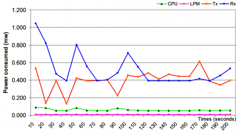
Table 4. Power consumption on TmoteSky 15

Note: See datasheet for TmoteSky pp.9 [1] 1. Active courant at Vcc = 500µA/s = 0.50mA/s, Voltage = 3v and 1s = 32768 clocks. 2. i.e. Energy consumed (CPU) = (34244-14902) × 0.50 × 3 / (32768 × 10) = 0,088541 mw.

Table 4 displays a return of Tmote Sky values in four states in the form of a number of clock ticks.

- ALL_CPU: The total (high) CPU (CPU in active mode).

- ALL_LPM: The total number of ticks in an LPM state (low power mode).

- ALL_Tx: The total number of ticks in the Tx (Transmit) state.

- ALL_Rx: The number of ticks in the Rx (Receive) state.

We calculate the energy consumption using the formula of Eq. (5).

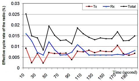
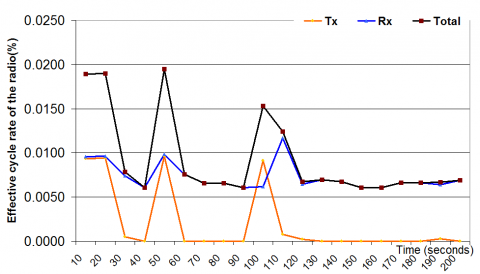
The standard model displays in Figure 5 the variation of the energy consumption in the four states mentioned previously. We can clearly see that the increase in energy concerns the transmission but above all the reception. Figure 6 confirms our assertion by summing the transmission and reception energies to represent the effective radio service cycle.

5.png

Figure 5. Skymote 15 power consummation in standard detection

6.png

Figure 6. Effective cycle rate of the radio after every 10 seconds from mote 15 in standard detection

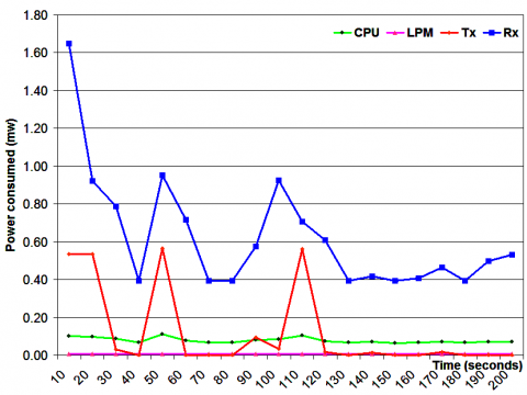
2. Mote 6: The data of Mote 6 in number of captured ticks are displayed in the following graph:

7.png

Figure 7. Skymote 6 power consummation in standard detection

As for Figure 5, Figure 7 represents the variation of the energy consumption in the four states (CPU, LPM, Tx, Rx) of the mote 6 in the standard model. Figure 8 shows the effective radio cycle in order to show the difference between emission and transmission.

8.png

Figure 8. Effective cycle of the radio after every 10 seconds from mote 6 in standard detection

9.png

Figure 9. Skymote 7 power consummation in standard detection

3. Mote 7: Now we are going to study the energetic behavior of mote 7.

Including its effective radio cycle in order to understand the influence of the distance of a mote from the sink in order to previously predict an optimal unfolding with collaboration the nodes between them. The data of word 7 in number of captured ticks are displayed in Figure 9. Just as Figures 5 and 7, Figure 9 shows the variation of the energy consumption in the four states (CPU, LPM, Tx, Rx) of the mote 7 in the standard model.

10.png

Figure 10. Effective cycle rate of the radio after every 10 seconds from mote7 in standard detection

By analyzing Figure 4 of the scenario of the topology of the standard detection model, we notice that the mote7 is outside the coverage of the sink on one side and that it has almost no neighbor. Figure 10 denotes a virtual absence of transmission but the mote6 is still listening.

4.2 Standard detection method discussion

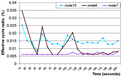
Note that mote 15 and mote 6 are in the same coverage of the sink (mote1), on the other hand mote 7 is outside the coverage area of the sink.

It can be seen in Figure 11 that the energy consumption by the three motes 15, 6 and 7 is more marked on the motes in packet reception mode (Rx) (Figures 5, 7 and 9), this could be explained by the fact that the motes are always listening to the transmission channel, and this is also proved by the results found by the effective cycle of each mote (high percentage of Rx compared to Tx).

11.png

Figure 11. Effective cycle rate of the radio comparison for of the three motes, after every 10 seconds in standard detection

12.png

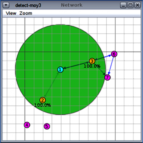
Figure 12. Scenario of a topology in the triple point method

The corresponding data on the eve of these three motes (mote 15, mote 6, mote 7) is represented by the parameter LPM which underlines an energy consumption. This means that the motes consume almost no power when they are in standby mode.

According to Figure 11, the use of the radio is more accentuated when the motes are on the cover of the sink, but it is much more when it approaches the latter. This could be explained by the fact that mote 15 is more likely to relay data to the sink than others. This deduction is also verified by analyzing the amount of energy consumed by CPU during processing. For example, mote 15 prints (Figure 5) an average usage between [0.3 mw - 0.5 mw].

An important remark is also verified from these results is the fact that when a mote (here mote6) has several neighbors, the energy consumed at reception increases considerably (Figure 6), this can be verified with mote 7 which has only one neighbor (mote17).

So, for an optimum deployment of the sensors, it is necessary to avoid the concentration of the nodes around a single mote because this could induce an excessive use of energy and arrive at its loss and a re-structuring of the topology or to permanently lose the network of sensors wireless.

4.3 Simulation with the triple point method

The configuration chosen is given by the following Figure 12. The simulation of our method is based on 7 motes. One sink, 4 standard catch motes and two aggregator motes responsible for cooperation to send a single value, according to a consensus, to the Sink.

Standard motes 4, 5, 6, 7 detect and transmit the values of temperature, humidity and light in broadcast. Motes 4 and 5 aggregate their data to word 2 and words 6 and 7 to word 3. Motes 2 and 3 are the aggregators.

Our method is based on aggregators to optimize radio transmission and overcome the problems posed by the standard configuration.

Once the simulation is triggered, the POWERTRACE tool gives the following results in Table 5:

1. Mote 2: On this mote we note the number of ticks after every 10 seconds:

Table 5. Number of ticks for a mote 2

13.png

Figure 13. Skymote 2 power consummation in the triple point method

By respecting the same approach of the standard model but using our algorithm this time, we obtain Table 5 representing the number of ticks in the four states (CPU, LPM, Tx, Rx) for the mote 2. Next, we calculate the energy consumption using the formula of the Eq. (4).

Next, we calculate the energy consumption using the formula of the Eq. (5) and after a graphical representation we obtain Figure 13 which visualizes the energy consumption by our triple point method. This curve highlights an increase in energy consumption around the radio (Tx, Rx).

Likewise, Figure 14 underlines a use much of the transmission than that of reception.

14.png

Figure 14. Percent of number of ticks for mote 2 in the triple point method

2. Mote 3: On this aggregator mote we note also the number of ticks after every 10 seconds:

Similarly to Mote 2 and by using the POWERTRACE tool, the data collected by the Mote 3 aggregator is shown in Figure 15 marking the energy consumed in transmission and reception as well as by the processor.

15.png

Figure 15. Skymote 3 power consummation in the triple point method

The energy consumption using the formula of the Eq. (5) and after a graphical representation we obtain Figure 16 which visualizes the energy consumption by our triple point method. This curve highlights an increase in energy consumption around the radio (Tx, Rx). Figure 16 displays the actual cycle of radio use and gives a graphical representation of high listening use versus transmission which appears occasional.

16.png

Figure 16. Percent of number of ticks for mote 3 in the triple point method

3. Mote 4: This is a simple sensor outside the sink coverage area and we want to follow its behavior and energy consumption throughout the process with the triple point method. Table 6 note also the number of ticks after every 10 seconds.

Figures 17 and 18 show the energy consumption of the main modules in Module 4 using the triple point method, respectively. The observation is highlighted on the receive (Rx) mode in front and the transmission thereafter.

Table 6. Number of ticks for a mote 4

17.png

Figure 17. Skymote 4 power consummation in the triple point method

4.4 Triple point method discussion

According to the above results, we notice that the energy consumption by the three motes when these motes are in transmission (TX) or reception (RX) mode is greater than that if these same motes are in calculation (CPU) or standby (LPM). This means that most of the energy is often consumed in transmitting and receiving, and it is consumed more in receiving than in transmitting.

18.png

Figure 18. Percent of number of ticks for mote 4 in the triple point method

19.png

Figure 19. Effective cycle rate of the radio comparison for of the three motes, after every 10 seconds in in the triple point method

In Figure 19, we compare the two motes 2 and 3 which serve as aggregators for a mote 4, we note that the latter consumes a lot of energy than the aggregators and this is explained by the transmissions of temperatures, humidity rates and humidity rates broadcast light every 10 seconds.

4.5 Comparison of the two methods

The standard protocol of the RPL Cooja makes it possible to relay the value captured from one mote to another in a normal way. This method is simple and does not require any calculation. But the values captured are not always reliable and can cause a false alarm and a waste of time and resources for an audit. We have suggested a new method based on a reliability consensus governed by an aggregator node. It is based on a collector which calculates the average, at most, of the first three values received, which then sends them to the Sink; this one we named it "the method of the triple points". This perspective ensures data reliability on one side and network perpetuity on the other side.

By taking the two plots of the effective radio cycles (Figures 11 and 19) side by side, we can draw the following conclusion:

(i) The maximum energy consumption by the standard method is 3.5% compared to our method which is 2.5%.

(ii) In our method the average consumption is around 1.1% compared to the standard method which exceeds 1.5% in energy.

(iii) It can also be noted that listening to the Rx reception channel is expensive in energy, but Tx transmission is more occasional.

(iv) In the standard method, mote 7 is not covered by the sink, so it is not overly stressed (no neighbor) if its reactivity will visibly increase the energy curve.

We notice that the standard RPL protocol gives very good results in response time but in power consumption it is by far the best. Our solution called 'triple points' is obviously the best solution in energy consumption and therefore the perpetuity of the network.

The standard method underlines a more interesting convergence time than our method that is surely due to our program for processing the average consensus but on the other hand it consumes more energy than ours.