Li Chen* | Jianfeng Ding
© 2021 IIETA. This article is published by IIETA and is licensed under the CC BY 4.0 license (http://creativecommons.org/licenses/by/4.0/).
OPEN ACCESS
Crispness is an important indicator of crunchy food. However, it cannot be easily quantified by sensory evaluation, due to the high subjectivity of evaluators; instrument measurement of this indicator requires much manpower and time. To improve the efficiency of food crispness prediction, this paper attempts to build a rapid, convenient, and accurate crispness analysis model. Starting with the fracturing sound of crunchy food, the authors collected the fracturing acoustic signal, conducted wavelet denoising, analyzed the eigenvalues in time and frequency domains, and constructed crispness prediction models based on multiple linear regression (MLR) and neural network, respectively. Through fracturing test and acoustic test, cluster analysis was adopted to select the typical eigenvalues of acoustic signal, including the peak amplitude of power spectral density (PSD) curve, amplitude difference, and waveform index. Based on these eigenvalues, a crispness analysis model was established, and used to predict the crispness of four kinds of food, namely, potato, sweet potato, carrot, and turnip. The results show that the BP neural network had a smaller relative error than the MLR; when the threshold was 5%, the BP neural network maintained a prediction accuracy of >90%, and achieved 100% prediction accuracy on two types of food. To sum up, this paper reveals the relationship between the food chewing sound features and food quality, laying the theoretical basis for the research of food chewing sound mechanism.
food crispness, acoustic signal, wavelet denoising, backpropagation (BP) neural network
In recent years, crunchy food has gained immense popularity among consumers, which kicks off a wave of research on crunchy food. Crispness, as an indicator of the freshness, maturity, and hygiene of food, directly reflects food quality. Sensory evaluation is a critical method to assess crispness. But this approach is susceptible to the preference, physical condition, and cultural difference of evaluators, and unable to quantify the value of crispness. The mechanics research on crispness mainly relies on the texture analyzer, which consumes much manpower, material, and time. To evaluate crispness, this paper tries to correlate the crispness with the food chewing sound features.
The research on the relationship between crunchy food quality and acoustic features can be traced back to the last century. Some of the latest researches are as follows: Dias-Faceto et al. [1] combined texture analyzer with acoustic detector to simulate our chewing of crunchy food and sense the food texture, and discovered the significance correlation between force curve parameters and acoustic curve parameters through experiments. Through three-point bending test and cutting test, Carsanba et al. [2] found that the number of force peaks and acoustic pressure peaks during food fracturing are strongly correlated with crispness. Zadeike et al. [3] learned that fast and nondestructive acoustic technology is an effective tool to monitor the food quality in the process of baking. From the angle of molecular motion, Roudaut et al. [4] explained the impact of moisture on bread crispness, and identified the direct relationship between the fracturing acoustic intensity and crispness. Chen et al. [5] developed a sound detector to detect the mechanical and acoustic curves at the fracturing of six types of biscuits, observed sudden pressure drops at the appearance of acoustic signal, and noticed the correlation between the second-order derivative of the mechanical curve and the acoustic curve, indicating that the energy of the biscuits is released to the air in the process of fracturing. Using a multifunctional texture analyzer, Taniwaki and Kohyama [6] analyzed the mechanical properties and acoustic features, and evaluated the crispness of potato chips, with a special focus on the acoustic features near the main fracture point; the results verified the assumption that the crispness of potato chips can be felt when the food completely fractures, and confirmed that the force drop at the fracture point has an obvious correspondence with the acoustic pressure. Costa et al. [7] carried out mechanics and acoustic detections on 86 different varieties of apples, extracted 16 mechanical and acoustic parameters for principal component analysis (PCA), and demonstrated the correlation between acoustic features and crispness. Arimi et al. [8] examined the crispness of biscuits with different moisture activities, revealing that the area under the acoustic curve in the time domain decreases with the crispness of the food.
Not many Chinese scholars have studied the quality and acoustic features of crunchy food. Yin [9] analyzed the correlation between acoustic signal features and hardness of apple, created an apple hardness prediction model based on acoustic features, and realized rapid nondestructive detection of apple hardness. Wang [10] discussed the acoustic features of carrot at fracturing, noted the good correlations between waveform index, signal strength, fracturing stress, fracturing energy, and elastic modulus, and then modeled the relationship between fracturing acoustic features of carrot.
The frequency domain map of the acoustic signal is very helpful for crispness detection. De Belie et al. [11] evaluated apple crispness by analyzing the amplitude, energy, and frequency in the chewing sound frequency domain map through fast Fourier transform (FFT). Srisawas and Jindal [12] analyzed the acoustic signal domain maps of several types of puffed food, and selected the eigenvalues for crispness evaluation.
A common way to determine the amplitude, frequency, and phase of sine wave is to convert time domain map to frequency domain map through Fourier transform [13, 14]. Wavelet denoising offers a popular and widely used tool to process frequency domain maps. Huang et al. [15] captured the frequency features of seismic waves accurately through wavelet denoising. Nguyen et al. [16] removed the noise from electrocardiogram signal, thereby eliminating contrasts and improving diagnosis accuracy. Khullar et al. [17] proposed a novel three-dimensional (3D) wavelet denoising algorithm, which removes the noise from functional magnetic resonance imaging (fMRI) data with the aid of wavelet transform and signal estimation theory. To enhance the weak echo signal of the laser radar, Xu et al. [18] reduced the noise amplitude through wavelet denoising, and established a probability detection model of laser radar.
In general, there is not yet a mature evaluation model of food quality based on chewing sound signal. Jessop et al. [19] studied the relationship between the electromyogram of masseter and acoustic curve during chewing, and constructed a feasible food quality evaluation model based on the features of the two curves. Zhang et al. [20] collected chewing sound signal of human, and developed a model to estimate food quality; But the model still requires a lot of manpower to quantify food quality.
The current evaluation methods for food crispness are largely fuzzy and subjective. There is no systematic, deep analysis of the acoustic features of crunchy food, not to mention quantifying the relationship between fracturing acoustic signal and crispness of food. Therefore, this paper presents a crispness prediction model based on chewing acoustic features. The work mainly covers five parts: collecting fracturing acoustic signal from crunch food; signal denoising; extracting eigenvalues in time and frequency domains, and analyzing their correlations with crispness; further screening of eigenvalues through cluster analysis; building prediction model. Based on acoustic signal features, the crispness prediction model saves the time, manpower, and material required for crispness evaluation, providing a rapid and convenient way to quantify the crispness of crunchy food.
2.1 Test materials
The test materials include potato, sweet potato, carrot, and turnip, all of which were purchased from a fruit and vegetable market.
2.2 Test instruments
The test instruments include CT3 texture analyzer, sound sensor, Lenovo laptop computer, Dell laptop computer, self-made sample table, and PHO70A drying box.
2.3 Test methods
The crispness was measured by texture analyzer through tests. The first peak on the force curve during the first compression was taken to characterize the stress on the food during fracturing.
To establish the relationship between the fracturing acoustic signal and crispness of each sample, the moisture gradient of each sample was configured, and the sample was dried. Firstly, each sample was divided into blocks of 2cm×1cm×1cm, and then dried for 5-10min at 60℃, until no acoustic signal was captured at the fracturing of the sample. In this way, 10 moisture gradients were obtained for potato, 8 for sweet potato, 7 for carrot, and 7 for turnip.
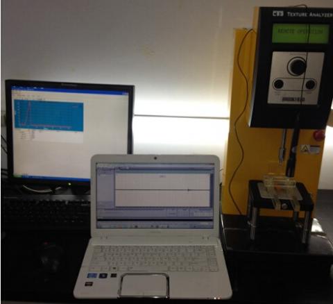
As shown in Figure 1, CT3 texture analyzer was selected for mechanical tests. The sensor was placed at 4cm away from the acoustic source. To mimic chewing, a bionic indenter was chosen as the probe [21]. During the tests, each sample was compressed only once at the speed of 1mm/s. The test distance was 6mm, and the trigger point load was 0.1N. Ten parallel tests were conducted on each sample.
Figure 1. Food crispness test instruments
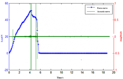
Figure 2. Force curve and time domain map of acoustic signal at sample fracturing
During the mechanical tests, the sensor was connected to the computers, and the acoustic signal was collected by Adobe Audition 3.0. The captured force map and acoustic map were merged into the same figure on MATLAB (Figure 2). It can be seen that the acoustic curve reached the highest amplitude, as the force curve arrived at its peak; the amplitude of acoustic signal gradually increased with the degree of compression. Hence, it was hypothesized that the crispness of a type of food can be perceived when the food completely fractures, and the acoustic signal have much to do with the force at the fracturing. Since the acoustic signal are related to force signal, which strongly correlate with perceived crispness, it is possible to predict food crispness based on acoustic signal.
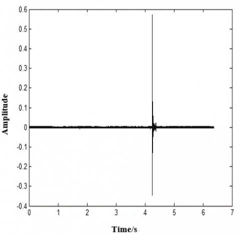
Figure 3. Time domain map of acoustic signal
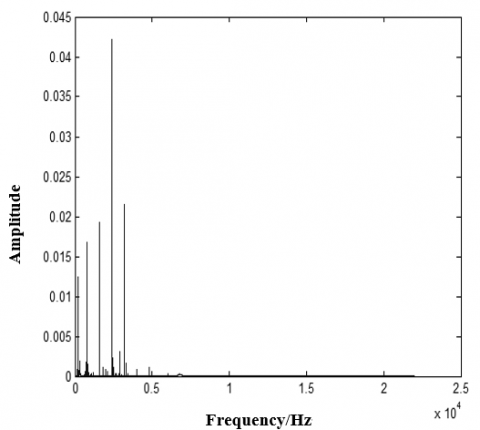
Figure 4. Frequency domain map of acoustic signal
The sample length of the sound card was set to 16bit. Figures 3 and 4 present the time and frequency domain maps of the collected acoustic signal, respectively.
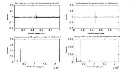
Wavelet denoising was performed on the acoustic signal with the default threshold. By the ddencmp function of MATLAB, the default threshold for the signal was obtained. Then, the original acoustic signal was subject to eight-layer wavelet decomposition, using db2 wavelet basis. Figure 5 shows the time and frequency domain effects of wavelet denoising.
Figure 5. Time and frequency domain maps of acoustic signal before and after wavelet denoising
As shown in Figure 5, the wavelet denoising reduced the noise in the original acoustic signal, making the signal purer, and revealed more characteristic peaks.
4.1 Selection of time domain features
(1) Extraction of time domain features
The following time domain features were acquired through MATLAB programming: signal strength, maximum short-term frame energy, amplitude difference, pulse factor, waveform index, and attenuation time.
The signal strength (unit: dB) refers to the total energy of the discrete acoustic signal at all sampling points. Let x(n) be the discrete acoustic signal. Then, the signal strength (E) can be calculated by:
$E={{\sum\limits_{n=0}^{N-1}{\left| x(n) \right|}}^{2}}$ (1)
where, N is the number of sampling points.
The maximum short-term frame energy (unit: dB) refers to the highest energy among the frames divided from the acoustic signal via FFT. Let x(n) be the time series of a frame of acoustic signal. Then, the maximum short-term frame energy (Emax) can be calculated by:
${{E}_{\max }}=\max {{\left| x(n) \right|}^{2}}$ (2)
The amplitude difference (unit: dB) refers to the difference between the maximum and minimum amplitudes of the acoustic signal in the time domain. Let x(n) be the discrete acoustic signal. Then, the amplitude difference (D) can be calculated by
$D=\max x(n)-\min x(n)$ (3)
The pulse factor refers to the ratio of the maximum amplitude to the absolute value of amplitude of the acoustic signal in the time domain. Let x(i) be the discrete acoustic signal. Then, the pulse factor (Y1) can be calculated by:
${{Y}_{1}}={x(n)}/{\left[ \frac{1}{N}\sum\limits_{i=0}^{N-1}{\left| x(i) \right|} \right]}\;$ (4)
where, x(n) is the maximum value of x(i).
The waveform index refers to the ratio of energy to root-mean-square of amplitude of the acoustic signal. The waveform index (Y2) can be calculated by:
${{Y}_{2}}={{{\sum\limits_{N=0}^{N-1}{\left| x(i) \right|}}^{2}}}/{\sqrt{\frac{1}{N}\left( \sum\limits_{i=0}^{N-1}{\left| x(i) \right|} \right)}}\;$ (5)
The attenuation time (unit: s) refers to the time for the acoustic signal to decay from the maximum amplitude to 0.1 times of the amplitude in the time domain. Let x1=max|x(n)| be the maximum amplitude of acoustic signal; l1 be the number of sampling points corresponding to x1; l2 be the number of sampling points corresponding to x2=0.1x1; fs be the sampling frequency. Then, the attenuation time (t) can be calculated by:
$t=\frac{{{l}_{2}}-{{l}_{1}}}{{{f}_{s}}}$ (6)
(2) Correlation analysis between time domain features of acoustic signal and food crispness
The above six time domain features were extracted from potato, sweet potato, carrot, and turnip with different crispness values. Then, the authors analyzed the correlations between these eigenvalues with food crispness. It was discovered that sample crispness is strongly correlated with signal strength, maximum short-term frame energy, amplitude difference and waveform index, but not clearly correlated with pulse factor or attenuation time. The correlation coefficients are listed in Table 1. Therefore, signal strength, maximum short-term frame energy, amplitude difference and waveform index were chosen as the final time domain features.
Table 1. Correlation coefficients between time domain features of acoustic signal and food crispness
|
|
Signal strength |
Maximum short-term frame energy |
Amplitude difference |
Pulse factor |
Waveform index |
Attenuation time |
|
Potato |
0.83 |
0.79 |
0.78 |
0.41 |
0.86 |
0.03 |
|
Sweet potato |
0.75 |
0.76 |
0.89 |
0.02 |
0.88 |
0.38 |
|
Carrot |
0.97 |
0.92 |
0.92 |
0.00 |
0.95 |
0.49 |
|
Turnip |
0.95 |
0.90 |
0.94 |
0.03 |
0.97 |
0.03 |
4.2 Selection of frequency domain features
(1) Extraction of frequency domain features
The time domain map of acoustic signal was converted into power spectral density (PSD) map through Fourier transform. The eigenvalues were extracted from the PSD map to analyze their correlation with food crispness. Through MATLAB programming, the following frequency domain features were obtained: peak PSD amplitude, peak location, PSD.
Let Ai be the amplitude of PSD curve. Then, the peak PSD amplitude (Xmax) can be calculated by:
${{X}_{\max }}=\max ({{A}_{i}})$ (7)
During the plotting process, the ordinate value of 10*log10(xi) was converted to the unit of dB. All ordinate values obtained were negative. Thus, the absolute value of the peak was chosen for correlation analysis against food crispness.
The peak location refers to the frequency corresponding to the peak PSD amplitude.
Let Ai be the amplitude of PSD curve. Then, the PSD (unit: dB) (G) can be calculated by:
$G=\sum\limits_{i=0}^{N-1}{{{A}_{i}}}$ (8)
(2) Correlation analysis between frequency domain features of acoustic signal and food crispness
Table 2. Correlation coefficients between frequency domain features of acoustic signal and food crispness
|
|
Peak PSD amplitude |
Peak location |
PSD |
|
Potato |
0.88 |
0.00 |
0.92 |
|
Sweet potato |
0.73 |
0.00 |
0.89 |
|
Carrot |
0.88 |
0.00 |
0.84 |
|
Turnip |
0.94 |
0.00 |
0.97 |
The above three frequency domain features were extracted from potato, sweet potato, carrot, and turnip with different crispness values. Then, the authors analyzed the correlations between these eigenvalues with food crispness. It was discovered that sample crispness is strongly correlated with peak PSD amplitude and PSD, but not correlated with peak location. The correlation coefficients are listed in Table 2. Therefore, peak PSD amplitude and PSD were chosen as the final frequency domain features.
The time and frequency domain features were further screened through system clustering. The clustering methods include inter-class clustering and clustering in R, using Pearson correlation coefficient. The screening results are presented in Figure 6.
Figure 6. Tree diagram of cluster analysis on time and frequency domain features
Figure 6 provides the three diagram of cluster analysis on time and frequency domain features for the acoustic signal. When the distance was set to 20, the eigenvalues fell into two classes: the first class includes peak PSD amplitude and PSD; the second includes amplitude difference, waveform index, maximum short-term frame energy, and signal strength.
When the distance was set to 15, the eigenvalues fell into three classes: the first class includes peak PSD amplitude and PSD; the second includes amplitude difference; the third includes signal strength, waveform index, and maximum short-term frame energy.
When the distance was set to 10, the eigenvalues fell into four classes: the first class includes PSD; the second includes peak PSD amplitude; the third includes amplitude difference; the fourth includes signal strength, waveform index, and maximum short-term frame energy.
When the distance was set to 5, the eigenvalues fell into five classes: the first class includes PSD; the second includes peak PSD amplitude; the third includes amplitude difference; the fourth includes signal strength; the fifth includes waveform index, and maximum short-term frame energy.
For the features allocated to the same class, the mean of the square of the correlation coefficient between each feature in a class and every other feature in the same class was calculated, and the maximum value was taken as the typical eigenvalue:
${{\overline{R}}^{2}}=\frac{\sum{{{r}^{2}}}}{m-1}$ (9)
where, r is the correlation coefficient between a feature in a class and another feature in that class; m is the number of features in the class.
After system clustering, the approximate matrix and clustering table were obtained (Table 3 and Table 4).
Table 3. Approximate matrix
|
Case |
Signal strength |
Maximum short-term frame energy |
Amplitude difference |
Waveform index |
Peak PSD amplitude |
PSD |
|
Signal strength |
1.000 |
.471 |
-.040 |
.502 |
-.088 |
-.402 |
|
Maximum short-term frame energy |
.471 |
1.000 |
.034 |
.913 |
-.312 |
-.491 |
|
Amplitude difference |
-.041 |
.032 |
1.000 |
.072 |
-.012 |
-.054 |
|
Waveform index |
.502 |
.913 |
.072 |
1.000 |
-.423 |
-.545 |
|
Peak PSD amplitude |
-.088 |
-.312 |
-.012 |
-.421 |
1.000 |
.361 |
|
PSD |
-.041 |
-.491 |
-.054 |
-.545 |
.362 |
1.000 |
Table 4. Clustering table
|
Order |
Cluster portfolio |
|
Cluster of first appearance |
Next order |
||
|
|
Cluster 1 |
Cluster 2 |
Coefficient |
Cluster 1 |
Cluster 2 |
|
|
1 |
2 |
4 |
.916 |
0 |
0 |
2 |
|
2 |
1 |
2 |
.487 |
0 |
1 |
4 |
|
3 |
5 |
6 |
.365 |
0 |
0 |
5 |
|
4 |
1 |
3 |
.022 |
2 |
0 |
5 |
|
5 |
1 |
5 |
-.293 |
4 |
3 |
0 |
The results of the above empirical formula show that, if the features are divided into two classes, waveform index and peak PSD amplitude should be chosen; if they are divided into three classes, peak PSD amplitude, amplitude difference, and waveform index should be chosen; if they are divided into four classes, PSD, peak PSD amplitude, amplitude difference, and waveform index should be chosen; if they are divided into five classes, PSD, peak PSD amplitude, amplitude difference, signal strength, and waveform index should be chosen. Through the analysis, the optimal eigenvalues could be obtained when the distance is shorter than 15. Thus, the final eigenvalues were chosen as: peak PSD amplitude, amplitude difference, and waveform index.
6.1 Multiple linear regression (MLR) model
(1) MLR model construction
MLR was performed on the eigenvalues of peak PSD amplitude, amplitude difference, and waveform index, which were obtained through system clustering. Then, the MLR equations for potato, sweet potato, carrot, and turnip can be obtained as:
${{y}_{1}}=88.166-0.782{{x}_{1}}-0.775{{x}_{2}}-0.043{{x}_{3}}$ (10)
${{y}_{2}}=111.482+0.105{{x}_{1}}-0.982{{x}_{2}}-0.447{{x}_{3}}$ (11)
${{y}_{3}}=127.842-0.145{{x}_{1}}-1.481{{x}_{2}}+5.031{{x}_{3}}$ (12)
${{y}_{4}}=52.313+0.416{{x}_{1}}-0.412{{x}_{2}}+2.431{{x}_{3}}$ (13)
where, x1 is waveform index; x2 is the peak PSD amplitude; x3 is the amplitude difference.
The MLR equations have significant linear correlations, when the significance level is 0.05. The chi-squared values (R2) of formulas (10)-(13) were obtained as 0.93, 0.92, 0.92, and 0.90, respectively.
(2) Model prediction results
By the MLR equations, the predicted values and relative errors of potato, sweet potato, carrot, and turnip were obtained (Table 5). As shown in Table 5, the relative error of crispness prediction for potato was 2.78% at the maximum and 0.63% at the minimum, averaging at 1.70%; the relative error of crispness prediction for sweet potato was 11.23% at the maximum and 0.18% at the minimum, averaging at 3.28%; the relative error of crispness prediction for carrot was 18.47% at the maximum and 0.91% at the minimum, averaging at 7.13%; the relative error of crispness prediction for turnip was 3.46% at the maximum and 0.18% at the minimum, averaging at 1.316%. Although the relative error was greater than the ideal relative error on a few samples, the prediction effect was acceptable for most samples.
Table 5. Prediction results of MLR equations
|
|
Sample number |
1 |
2 |
3 |
4 |
5 |
6 |
7 |
8 |
9 |
10 |
|
Potato |
Actual value (N) |
28.38 |
33.38 |
35.71 |
38.11 |
39.82 |
42.96 |
45.02 |
47.94 |
49.32 |
54.22 |
|
Predicted value (N) |
28.56 |
33.75 |
34.88 |
38.97 |
40.33 |
41.81 |
45.34 |
46.95 |
48.77 |
55.73 |
|
|
Relative error (%) |
0.63 |
1.11 |
-2.32 |
2.26 |
1.29 |
-2.68 |
0.71 |
-2.07 |
-1.12 |
2.78 |
|
|
Sweet potato |
Actual value (N) |
30.46 |
40.12 |
45.29 |
47.43 |
50.37 |
54.34 |
59.29 |
64.75 |
68.56 |
71.68 |
|
Predicted value (N) |
33.88 |
40.96 |
44.48 |
46.08 |
50.46 |
52.83 |
61.28 |
62.23 |
66.18 |
70.82 |
|
|
Relative error (%) |
11.23 |
2.09 |
-1.79 |
-2.85 |
0.18 |
-2.78 |
3.36 |
-3.89 |
-3.47 |
-1.20 |
|
|
Carrot |
Actual value (N) |
17.64 |
19.65 |
22.12 |
27.59 |
28.25 |
36.25 |
39.53 |
40.78 |
50.43 |
55.53 |
|
Predicted value (N) |
15.49 |
23.28 |
25.27 |
28.57 |
30.42 |
33.98 |
37.89 |
40.41 |
45.52 |
53.42 |
|
|
Relative error (%) |
-12.2 |
18.47 |
14.24 |
3.55 |
7.68 |
-6.26 |
-4.15 |
-0.91 |
9.73 |
3.8 |
|
|
Turnip |
Actual value (N) |
17.71 |
21.37 |
23.25 |
24.92 |
28.38 |
30.08 |
32.52 |
37.82 |
38.96 |
41.96 |
|
Predicted value (N) |
18.05 |
21.31 |
23.18 |
25.43 |
28.43 |
31.12 |
33.08 |
37.53 |
39.65 |
41.71 |
|
|
Relative error (%) |
1.92 |
-0.28 |
-0.3 |
2.05 |
0.18 |
3.46 |
1.72 |
-0.77 |
1.77 |
-0.6 |
Table 6. Prediction results of BP neural network
|
|
Sample number |
1 |
2 |
3 |
4 |
5 |
6 |
7 |
8 |
9 |
10 |
|
Potato |
Actual value (N) |
28.38 |
33.38 |
35.71 |
38.11 |
39.82 |
42.96 |
45.02 |
47.96 |
49.32 |
54.22 |
|
Predicted value (N) |
29.11 |
33.85 |
35.92 |
37.32 |
40.11 |
42.97 |
44.81 |
47.41 |
49.28 |
52.86 |
|
|
Relative error (%) |
2.57 |
1.41 |
0.59 |
2.08 |
0.73 |
0.02 |
0.47 |
1.15 |
0.08 |
2.51 |
|
|
Sweet potato |
Actual value (N) |
30.44 |
40.12 |
45.27 |
47.43 |
50.35 |
54.32 |
59.29 |
64.75 |
68.54 |
71.68 |
|
Predicted value (N) |
32.88 |
41.36 |
45.54 |
46.75 |
52.32 |
54.16 |
59.83 |
63.82 |
68.44 |
70.06 |
|
|
Relative error (%) |
8.02 |
3.09 |
0.6 |
1.43 |
3.91 |
0.29 |
0.91 |
1.44 |
0.15 |
2.26 |
|
|
Carrot |
Actual value (N) |
17.64 |
19.65 |
22.12 |
27.59 |
28.23 |
36.22 |
39.53 |
40.76 |
50.43 |
55.53 |
|
Predicted value (N) |
16.56 |
18.73 |
22.68 |
27.72 |
30.53 |
35.42 |
41.01 |
42.34 |
50.52 |
56.05 |
|
|
Relative error (%) |
-6.12 |
-4.68 |
2.53 |
0.47 |
8.15 |
-2.21 |
3.74 |
3.88 |
0.18 |
0.94 |
|
|
Turnip |
Actual value (N) |
17.89 |
21.36 |
23.23 |
24.92 |
28.38 |
30.08 |
32.53 |
37.92 |
38.95 |
41.98 |
|
Predicted value (N) |
18.08 |
21.58 |
23.2 |
25.31 |
28.63 |
30.68 |
32.38 |
38.99 |
40.17 |
41.46 |
|
|
Relative error (%) |
1.06 |
1.03 |
-0.13 |
1.57 |
0.88 |
1.99 |
-0.46 |
2.82 |
3.13 |
-1.24 |
6.2 BP neural network
(1) BP neural network construction
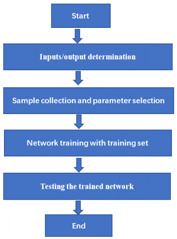
Figure 7 explains the workflow of prediction by BP neural network. The number of hidden layer nodes directly affects the performance of the BP neural network. Here, this number is determined in two steps: narrowing down the range of the number by empirical formula; determining the number through trial and error.
Since there are 3 nodes on the input layer and 1 on the output layer, the number of hidden layer nodes was limited to [1, 12] by empirical formula. Then, the number was finalized by comparing the mean squared errors (MSEs) of the network with different number of hidden layer nodes. In this way, the number of hidden layer nodes was determined as 10, 12, 12, and 7 for the BP neural networks of potato, sweet potato, carrot, and turnip, respectively. Through trail and error, the total number of nodes in the network was set to 100.
Figure 7. Workflow of BP neural network
(2) Model prediction results
By the BP neural network, the predicted values and relative errors of potato, sweet potato, carrot, and turnip were obtained (Table 6).
As shown in Table 6, the relative error of crispness prediction for potato was 2.57% at the maximum and 0.02% at the minimum, averaging at 1.16%; the relative error of crispness prediction for sweet potato was 8.02% at the maximum and 0.15% at the minimum, averaging at 2.21%; the relative error of crispness prediction for carrot was 8.15% at the maximum and 0.18% at the minimum, averaging at 3.29%; the relative error of crispness prediction for turnip was 3.13 % at the maximum and 0.13% at the minimum, averaging at 1.43%. Judging by the relative errors, BP neural network performed better than MLR in prediction.
6.3 Comparison between the two models
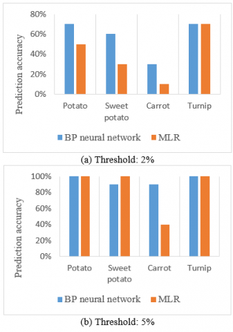
To find the better model for predicting sample crispness, the MLR model and BP neural network were separately applied to predict the crispness of 10 groups of samples. Each group was predicted by each model three times, and the mean of the three predictions was taken as the final result. To evaluate the prediction accuracy of each model, the threshold of relative error was set to 2% and 5% in turn (Figure 8).
Figure 8. Prediction accuracies of the two models
As shown in Figure 8, BP neural network achieved better prediction results than the MLR model in most cases. When BP neural network was selected, the prediction effect was better at the relative error threshold of 5%: the prediction accuracy was as high as 90% for sweet potato and carrot, and 100% for potato and turnip.
This paper constructs crispness prediction models for potato, sweet potato, carrot, and turnip based on their fracturing acoustic features. The main conclusions are as follows:
(1) For the MLR model, when the threshold of relative error was set to 2%, the prediction accuracy was 50% for potato, 30% for sweet potato, 10% for carrot, and 70% for turnip; when the threshold of relative error was set to 5%, the prediction accuracy was 100% for potato, 100% for sweet potato, 40% for carrot, and 100% for turnip.
(2) For the BP neural network, when the threshold of relative error was set to 2%, the prediction accuracy was 70% for potato, 60% for sweet potato, 30% for carrot, and 70% for turnip; when the threshold of relative error was set to 5%, the prediction accuracy was 100% for potato, 90% for sweet potato, 90% for carrot, and 100% for turnip.
The above data show that BP neural network with the relative error threshold of 5% was the optimal model for predicting food crispness.
This work is supported by Science and Technology Research Planning Project, Department of Education, Jilin Province, China (Grant No.: JJKH20210177KJ).
[1] Dias-Faceto, L.S., Salvador, A., Conti-Silva, A.C. (2020). Acoustic settings combination as a sensory crispness indicator of dry crispy food. Journal of Texture Studies, 51(2): 232-241. https://doi.org/10.1111/jtxs.12485
[2] Çarşanba, E., Duerrschmid, K., Schleining, G. (2018). Assessment of acoustic-mechanical measurements for crispness of wafer products. Journal of Food Engineering, 229: 93-101. https://doi.org/10.1016/j.jfoodeng.2017.11.006
[3] Zadeike, D., Jukonyte, R., Juodeikiene, G., Bartkiene, E., Valatkeviciene, Z. (2018). Comparative study of ciabatta crust crispness through acoustic and mechanical methods: Effects of wheat malt and protease on dough rheology and crust crispness retention during storage. LWT, 89: 110-116. https://doi.org/10.1016/j.lwt.2017.10.034
[4] Roudaut, G., Dacremont, C., Le Meste, M. (1998). Influence of water on the crispness of cereal-based foods: Acoustic, mechanical, and sensory studies. Journal of Texture Studies, 29(2): 199-213. https://doi.org/10.1111/j.1745-4603.1998.tb00164.x
[5] Chen, J., Karlsson, C., Povey, M. (2005). Acoustic envelope detector for crispness assessment of biscuits. Journal of Texture Studies, 36(2): 139-156. https://doi.org/10.1111/j.1745-4603.2005.00008.x
[6] Taniwaki, M., Kohyama, K. (2012). Mechanical and acoustic evaluation of potato chip crispness using a versatile texture analyzer. Journal of Food Engineering, 112(4): 268-273. https://doi.org/10.1016/j.jfoodeng.2012.05.015
[7] Costa, F., Cappellin, L., Longhi, S., Guerra, W., Magnago, P., Porro, D., Gasperi, F. (2011). Assessment of apple (Malus × domestica Borkh.) fruit texture by a combined acoustic-mechanical profiling strategy. Postharvest Biology and Technology, 61(1): 21-28. https://doi.org/10.1016/j.postharvbio.2011.02.006
[8] Arimi, J.M., Duggan, E., O’sullivan, M., Lyng, J.G., O’riordan, E.D. (2010). Effect of water activity on the crispiness of a biscuit (Crackerbread): Mechanical and acoustic evaluation. Food Research International, 43(6): 1650-1655. https://doi.org/10.1016/j.foodres.2010.05.004
[9] Yin, M. (2019). Research on rapid detection method and device of apple hardness based on acoustic characteristics. Shandong Agricultural University.
[10] Wang, X. (2017). Characteristics of mechanical acoustic behavior and Micromorphology of carrot. Jilin University.
[11] De Belie, N., Harker, F.R., De Baerdemaeker, J. (2002). Ph-postharvest technology: Crispness judgement of royal gala apples based on chewing sounds. Biosystems Engineering, 81(3): 297-303. https://doi.org/10.1006/bioe.2001.0027
[12] Srisawas, W., Jindal, V.K. (2003). Acoustic testing of snack food crispness using neural networks. Journal of texture studies, 34(4): 401-420. https://doi.org/10.1111/j.1745-4603.2003.tb01072.x
[13] Taniwaki, M., Hanada, T., Sakurai, N. (2006). Device for acoustic measurement of food texture using a piezoelectric sensor. Food Research International, 39(10): 1099-1105. https://doi.org/10.1016/j.foodres.2006.03.010
[14] Maruyama, T.T., Arce, A.I.C., Ribeiro, L.P., Costa, E.J.X. (2008). Time–frequency analysis of acoustic noise produced by breaking of crisp biscuits. Journal of Food Engineering, 86(1): 100-104. https://doi.org/10.1016/j.jfoodeng.2007.09.015
[15] Huang, D., Cui, S., Li, X. (2019). Wavelet packet analysis of blasting vibration signal of mountain tunnel. Soil Dynamics and Earthquake Engineering, 117: 72-80. https://doi.org/10.1016/j.soildyn.2018.11.025
[16] Nguyen, T.N., Nguyen, T.H., Ngo, V.T. (2020). Artifact elimination in ECG signal using wavelet transform. Telkomnika, 18(2): 936-944. https://doi.org/10.12928/telkomnika.v18i2.14403
[17] Khullar, S., Michael, A., Correa, N., Adali, T., Baum, S. A., Calhoun, V.D. (2011). Wavelet-based fMRI analysis: 3-D denoising, signal separation, and validation metrics. Neuroimage, 54(4): 2867-2884. https://doi.org/10.1016/j.neuroimage.2010.10.063
[18] Xu, X., Luo, M., Tan, Z., Pei, R. (2018). Echo signal extraction method of laser radar based on improved singular value decomposition and wavelet threshold denoising. Infrared Physics & Technology, 92: 327-335. https://doi.org/10.1016/j.infrared.2018.06.028
[19] Jessop, B., Sider, K., Lee, T., Mittal, G.S. (2006). Feasibility of the acoustic/EMG system for the analysis of instrumental food texture. International Journal of Food Properties, 9(2): 273-285. https://doi.org/10.1080/10942910600596399
[20] Zhang, H., Lopez, G., Tao, R., Shuzo, M., Delaunay, J. J., Yamada, I. (2012). Food Texture Estimation from Chewing Sound Analysis. In HEALTHINF, 213-218. https://doi.org/10.5220/0003771802130218
[21] Chen, L., Sun, Y.A., Liu, J.J., Xie, G.P. (2014). Influence of bionic indenter on food 'texture based on electromyographic signal. Journal of agricultural machinery, 45(08): 248-253, 281. https://doi.org/10.6041/j. issn.1000-1298.2014.08.040