Jingfei Dong | Xun Li*
© 2020 IIETA. This article is published by IIETA and is licensed under the CC BY 4.0 license (http://creativecommons.org/licenses/by/4.0/).
OPEN ACCESS
The boom of global economy has caused an explosive growth in the issuance and use of financial instruments. Traditionally, the financial instruments are recognized and classified manually, which increases the burden of financial staff and consumes lots of financial time. To solve the problems, this paper designs a convolutional neural network (CNN) for classification of financial instruments, covering components like traditional CNN, shallow convolutional layers, and cropping structure. Then, the momentum weight update was combined with weight attenuation to accelerate the model learning. In addition, the authors designed a preprocessing method for rapid pixel-level adjustment of financial instruments, enabling the proposed CNN to classify financial instruments of various sizes. Experiments show that our CNN can identify various financial instruments, and classify them at an accuracy as high as 96%.
financial instruments, convolutional neural network (CNN), image classification, momentum weight update, weight attenuation
The computing power explosion has promoted the application of computer vision in various fields [1, 2]. One of the important application fields is the identification and classification of financial instruments [3]. Traditionally, these instruments are identified and classified manually by financial personnel in the following steps: First, various types of financial instruments are classified manually, including VAT (ordinary bills, electronic bills, special bills), bank receipts, toll bills (road invoice, charges, highway tolls). Then, the basic information of these financial products is manually input to the financial software to generate the corresponding accounting slip. After that, the accounting vouchers were attached to each financial instrument in turn; Finally, the financial personnel check and confirm the classification three to four times [4, 5]. The above method is undoubtedly inefficient. Considering the diversity and sheer number of financial instruments nowadays, the manual method will incur a heavy workload, and consume too much time in image classification [6, 7].
The traditional methods for image feature extraction mainly adopt such techniques as intensity histogram, feature-based filter, scale-invariant feature transform (SIFT), local binary pattern (LBP), and support vector machine (SVM) [8]. These techniques cannot accurately recognize images with highly complex scenes, and require a long time for model learning. As a computer vision technique, convolutional neural network (CNN) has achieved a good performance in image classification, due to its ability to describe and extract features.
For many years, artificial neural networks (ANNs) have been widely used to solve image classification and complex classification problems. The CNN is one of the most successful ANNs, because it has good performance in handling many problems of image classification. The defining feature of the CNN is the use of convolutional layers, which truthfully simulates the optic nerves of human. Each node can only respond to a specific image feature, such as horizontal or vertical edges. These simple nodes are arranged layer by layer. Sufficient features can be acquired by enough layers of nodes. Mimicking the human vision mechanism, the CNN boasts a good effect on image recognition. In some innovative applications, such as traffic sign detection, CNN-based systems are better than human vision in benchmark tests [9].
When it comes to the recognition and classification of financial instruments, the CNN also has super-strong control capability of the processing accuracy [10]. Therefore, this paper designs a CNN for the classification of financial instruments. The CNN consists of components like traditional CNN, shallow convolutional layers, and cropping structure. Then, the momentum weight update was combined with weight attenuation to accelerate the model learning. In addition, a preprocessing method was developed for rapid pixel-level adjustment of financial instruments, such that the proposed CNN can classify financial instruments of various types.
So far, many scholars have studied financial business processing and application based on machine learning. For example, Artaud et al. [11] adopted a local matching method, which only recognizes and classifies part of the input images on bank receipts. The authors applied the supervised taxonomy to each layout structure defined in Ma et al. [12] visual similarity, using various image features: percentages of graphs, images, tables, content areas, and regular structures, relative size of fonts, density of content areas, and statistical properties of connected components. Ding et al. [13] proposed an inter-page similarity estimation model for ordered image sets. Pham et al. [14] presented a banknote recognition system through the extraction and flexible matching of important pixels. Kaur et al. [15] discussed the general problem of using attributed relational graphs to classify the genre of printed images, represented the layout structure of document instances with parameters, and illustrated image types with a first-order random graph. Suyts et al. [16] used an k-means-based classifier to classify the forms of bank receipts, and divided the tax bills in the NIST Structured Forms Database by low-level pixel density and adaptive enhancement; nevertheless, their strategy could not classify financial business images, or handle different kinds of financial instruments at the same time.
The CNN is a proven method for image classification [17]. The CNN-based studies have achieved excellent results on mainstream databases, such as MNIST, NORB, and CIFAR10. Traditional image objects, such as handwritten numbers or faces, have local structural characteristics or global structural characteristics. Simple things, such as edge curves, can be combined into extremely complex features, such as shapes and angles. Recently, the CNN has been introduced to the analysis of financial instruments, e.g., tax bill identification and bill classification [18]. In this research, a CNN is developed specifically for the image classification of multi-class financial instruments, without invoking overfitting.
The overall architecture of our CNN is shown in Figure 1. The input to the network is normalized image blocks of financial instruments with a zero mean unit variance. The first layer is a convolutional layer with 16 output channels and a kernel size of 7×7 pixels. The second layer is the 2×2 pooling layer with the maximum kernel size. The third layer is a completely connected layer with 100,50 layers, and 5 nodes, respectively. The last layer is activated by softmax function.
Figure 1. The overall architecture of our CNN
Compared with CNN for other applications, our CNN involves multiple convolutional layers, and receives multi-class images. Thus, the network must be trained with largescale or high-level features. For the classification of financial instruments, a network with a limited number of convolutional layers has the same performance as a deep CNN. The simple structure greatly reduces the number of training parameters, which helps avoid overfitting. Besides, many techniques that improve or accelerate the network training were implemented. The learning parameters of these techniques were set to typical values or selected empirically. Each layer of the CNN is detailed in the following subsections.
3.1 Convolution-based extraction of image features
To solve the image classification problem, the input to the standard feedforward neural network can be used directly based on image pixels. But even a small image block may contain thousands of pixels, that is, numerous connection weights need to be trained. According to the theory on multi-dimensional data processing, too many weight parameters will complicate the system. In this case, more training samples are required to avoid overfitting. By combining the weights into small kernel filters, the CNN substantially simplifies the learning model, and operates faster and better than the traditional fully-connected neural network.
3.2 Convolutional layer
In image classification, convolutional layer is an important part of CNN. The number of input and output matrices may differ. One or more two-dimensional (2D) matrices serve as inputs to the convolutional layer, and the convolutional layer outputs multiple two-dimensional matrices. The calculation of a single output matrix can be defined as:
$A_{j}=f\left(\sum_{i=1}^{N} I_{i} * K_{i, j}+B_{j}\right)$ (1)
First, the corresponding kernel matrix Ki,j is convolved with each input matrix Ii and then summed, and the nonlinear activation function f(•) is added to the deviation Bj and applied to each element of the obtained matrix to obtain the output matrix Aj, and the features extracted by the local feature extractor represented by each set of kernel matrices are extracted from the input matrix. Finally, a set of kernel matrices K, is found and used to extract good discriminative features to classify the images. The connection weights of the CNN are optimized by the inverse algorithm, and the deviations and matrices are trained into network nodes with shared connection weights.
3.3 Max pooling layer
The pooling layer is responsible for dimensionality reduction of the CNN. In order to reduce the output nodes of the convolutional layer, the pooling algorithm was adopted to combine adjacent elements in each matrix outputted by the convolutional layer. Max pooling and average pooling are common pooling algorithm. In this research, a pooling layer with 2×2 kernels were adopted to select the maximum of the four adjacent elements in the output matrix usually selects the largest of the four adjacent elements in the input matrix. The gradient signal is used only for the nodes of the pool output, if the transmission is wrong.
3.4 Rectified linear unit (ReLU) activation
Neural networks often employ nonlinear transfer functions as the activation function of nodes. The sigmoid function f(x)=1/(1+e−x) and the hyperbolic tangent function f(x)=tanh(x) are commonly used activation functions. Both are saturated nonlinear functions: The output gradient decreases and approaches zero as the input increases. To improve learning speed and classification performance, our CNN adopts the latest activation function Mish [19]: f(x)=x*tanh(ln(1+ex)) [20], and applies it to the convolutional layer. Experimental evidence shows that Mish activation function has a faster convergence rate and a higher classification performance of 2.5% than the sigmoid activation function.
3.5 Backpropagation
Multiple techniques were adopted to accelerate and stabilize the CNN training, such as batch processing, momentum weight update, and weight attenuation. The authors batch processed 128 input samples, and the batch method was chosen to improve learning efficiency and accuracy, rather than updating the connection weights after each backpropagation, and their connection weights were updated at once.
To accelerate learning speed, weight attenuation update was coupled with momentum weight to update weight Δωi into:
$\Delta \omega_{i}(t+1)=\omega_{i}(t)-\mu \frac{\partial E}{\partial w_{i}}+\alpha \Delta \omega_{i}(t)-\lambda \mu \omega_{i}$ (2)
where, $\omega_{i}(t)-\mu \frac{\partial E}{\partial w_{i}}$ is the standard backpropagation term; $\omega_{i}(t)$ is the current weight vector; $\frac{\partial E}{\partial w_{i}}$ is the error gradient relative to the weight vector; μ is the learning rate; $\alpha \Delta \omega_{i}(t)$ is the momentum part; $\alpha$ is the momentum rate; $\lambda \mu \omega_{i}$ is the weight attenuation part; λ is the weight attenuation rate. In order to speed up learning, the authors made the momentum weight update, while the weight attenuation stabilizes the learning by slightly reducing the weight vector in each iteration. In our experiments, the learning rate, momentum rate, and weight attenuation rate were set to 0.001, 0.9, and 0.01, respectively, for each layer. These parameter values were determined through repeated experiments.
3.6 DropOut
The network performance was improved by randomly disabling nodes in each layer [21]. At the beginning of each training iteration, a DropOut with the same size of nodes was initialized in each layer to label the on or off state of the corresponding nodes. In the iterative training process, different models are switched in each learning iteration to train different models at the same time, and non-state nodes are removed from the network by disabling forward propagation of activation signals of nodes and wrong back propagation. During the test phase, all nodes are activated, but during the training phase, the activation signal decays to the average open rate. In our experiments, the DropOut was set to 0.6 for the training.
The images on financial instruments are digitized by scanning or photographing financial instruments. During image acquisition, two prominent issues arise to the features and complexity of financial instruments:
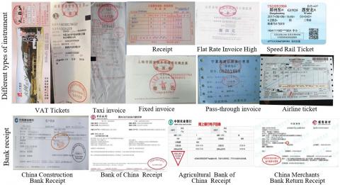
(1) There are various types of financial instruments (Figure 2), such as value-added tax invoices (bill, electronic bill, and special bill), bank receipts, toll bills (tickets, occupancy fees, and highway tolls), financial receipts, fiscal receipts, tourist attractions tickets, air tickets, train tickets, taxi tickets, and toll invoices. As a result, the financial instruments are extremely complex. For example, the 4,034 registered banks in China adopt different business vouchers with different styles.
(2) The image quality varies significantly (Figure 2), under the effects of multiple factors, namely, the quality of instrument, the model of collection device, technical differences, and factors in accidental collection. The main defects of image quality include wear, deformation, wrinkling, character overlap, tilt, obscuration, incompleteness, and complex background with uneven lighting.
Figure 2. The different types of financial instruments
Therefore, it is a great challenge to develop a highly adaptive and accurate intelligent recognition system for financial instruments. The system must realize the following functions: efficient and accurate classification of instruments, accurate identification and confirmation of instruments, correct recognition of instrument content, and correct recording of instruments. Before that, the instruments must be preprocessed through traditional methods like segmentation, correction, and enhancement [22]. Image processing and machine learning have contributed greatly to realizing these functions.
Lacking effective affine transform and projection, the traditional algorithms cause severe deformation to the instruments, such as wrinkling, character overlap, and breakage, and have a low accuracy in the recognition of financial instruments. Moreover, the limited capacity of existing methods cannot satisfy the needs for recognizing multiple and diverse instruments.
To realize the above functions, this paper designs a preprocessing method for rapid pixel-level adjustment of financial instruments. Each original image was continuously down-sampled until reaching the preset stopping point (which might be a single-pixel image), forming a pyramid image set. Then, each image was convolved with Gaussian kernels, and the even numbered rows and column were removed, producing the (i+1)-th layer of the pyramid from the i-th layer. In this case, the area of each image is exactly a quarter of its original area. The above process was implemented iteratively on the input images to create the entire pyramid. Each phase of pyramid generation was realized on OpenCV [23]. The target size was set to the default input size of our CNN: 32*32; the output image size was strictly controlled to half the size of the original image.
Specifically, an image set was created by calling function cv:: buildPyramid():
void cv::buildPyramid(cv::InputArray src, cv::OutputArrayOfArrays dst, int maxlevel)
where, src is the original image;
dst is an OutputArrayOfArrays, which can be regarded as an object of type STL vector<> or OutputArray; the most common example is vector <cv:: Mat>;
maxlevel is a random positive integer indicating the number of layers of the pyramid, i.e., the total number of images in the pyramid.
During the operation, buildPyramid() returns a vector in dst with the length of maxlevel + 1. The first item in dst will be the same as src; the second one will be half, just like that after calling pyrDown(); the third one will be half of the second.
Next, pyrUp() operation was called to convert the existing image into an image twice as large in each direction:
void cv::pyrUp(cv::InputArray src,cv::OutputArray dst,const cv::Size& dstsize = cv::Size ());
In this case, the image was first doubled in each dimension, and the new rows were filled with 0. After that, the missing pixels were estimated through convolution by a Gaussian filter.
5.1 Experimental settings
During the experiments, SIFT [24], LBP [25], and SVM were taken as the benchmarks to accurately monitor the recognition accuracy, computing speed, and operation state of our CNN in intelligent recognition and classification of financial instruments, without any manual intervention.
Our CNN model was established under the PyTorch framework, and deployed on the server operating system CentOS Linux 7. Two Nvidia Tesla v100 graphic cards, each with32G video memory, and a central processing unit (CPU) of 2.20GHz were adopted.
The multi-class financial instruments dataset was established through long-term collection and sorting of images on Google and Baidu, and the cooperation with financial institutions, as well as transportation and taxation departments. The 100,000 plus real instruments in the dataset were divided into 482 subclasses in 12 classes. The name and subclass number of the 12 classes are presented in Table 1. A total of 100 images were selected from each class and combined into a test set of 1,200 images, which cover financial instruments like value-added tax invoices, toll bills, quota tax invoices, train tickets, taxi invoices, and bank receipts.
Table 1. The name and subclass number of each class of financial instruments
|
|
Name |
Subclass number |
|
1 |
Bank receipt |
149 |
|
2 |
Value-added tax invoice |
104 |
|
3 |
Fee ticket |
85 |
|
4 |
Quota invoice |
51 |
|
5 |
Admission ticket |
25 |
|
6 |
Normal printed ticket |
21 |
|
7 |
Taxi invoice |
21 |
|
8 |
Air ticket |
11 |
|
9 |
Train ticket |
11 |
|
10 |
Insurance documents |
7 |
|
11 |
Receipt |
2 |
|
12 |
Others |
15 |
5.2 Results analysis
In our dataset, the images on financial instruments are collected by various methods from different sources. Some images contain multiple instrument areas and multiple instrument samples, while some only contain a single instrument area with a large background area. These factors impede the classification and recognition of images.
The images containing multiple instrument areas were adopted to verify the performance of our model. As shown in Figure 3, the classification accuracy averaged at 97%, indicating that our model has a good learning ability that mines the feature difference between instruments. The results also testify the reliability and practicability of the collected images.
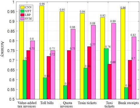
Further, the classification results of our method were compared with those of the other three feature extraction methods in terms of classification accuracy. According to Figure 4 that the CNN achieved the best classification performance. In support vector machines, feature learning is independent of classifier training. Compared with support vector machines, this method shows the superiority of supervised learning. In addition, compared with the currently popular feature descriptors SIFT and LBP, our CNN model has obvious advantages, which indicates the feasibility of automatic learning of financial instrument image features. The main advantages of our approach include the customization adaptability of CNN, and the fast preprocessing of instrument data, which are rare in current image calculation. Moreover, the neural network in classification model learning also contributes to the superiority of our method: the final classification model is optimized through parameter finetuning on each layer by backpropagation algorithm.
Figure 3. The classification effects on multiple instrument areas
Figure 4. The classification performance of different methods on financial instruments
Table 2. The training time of different methods
|
|
CNN |
SIFT |
LBP |
SVM |
|
Training time |
62,221s |
88,752s |
125,542s |
588,621s |
Table 2 records the training time of different methods. It can be seen that our method consumed 10 times shorter time in training than SVM. The training time of our method was even shorter than that of SIFT, which is known for its low complexity. The time efficiency comes from two unique properties: the simple structure of our model greatly facilitates training; the model learning is accelerated by the combination between momentum weight update and weight attenuation.
This paper proposes a customized CNN to classify the images on financial instruments. The designed convolutional layer can effectively learn features of different classes from training samples, and obtain good classification results. During the experiments, our CNN could adapt to the needs of image classification for financial instruments, despite the limited size of the training set. The results show that our CNN can automatically extract the discriminative features, without manual feature engineering, and achieve better performance than the benchmark algorithms.
This work is funded by Chongqing Social Science Fund Project (Grant No.: 2020YBJJ161), and Science and Technology Project of Chongqing Municipal Education Commission (Grant No.: KJ1707187).
[1] Yindumathi, K.M., Chaudhari, S.S., Aparna, R. (2020). Analysis of image classification for text extraction from bills and invoices. 2020 11th International Conference on Computing, Communication and Networking Technologies (ICCCNT), Kharagpur, India, pp. 1-6. https://doi.org/10.1109/ICCCNT49239.2020.9225564
[2] Zhang, H., Dong, B., Feng, B., Yang, F., Xu, B. (2020). Classification of financial tickets using weakly supervised fine-grained networks. IEEE Access, 8: 129469-129477. https://doi.org/10.1109/ACCESS.2020.3007528
[3] Huang, Z., Qian, L., Sun, S., Cai, D., Hang, T., Feng, Q. (2020). Design of dynamic cooperative robot system for financial bill recognition. 2020 4th International Conference on Automation, Control and Robots (ICACR), Rome, Italy, pp. 44-47. https://doi.org/10.1109/ICACR51161.2020.9265492
[4] Li, H., Huang, C., Gu, L. (2020). Image pattern recognition in identification of financial bills risk management. Neural Computing and Applications, 1-10. https://doi.org/10.1007/s00521-020-05261-3
[5] Smith, K.P., Kang, A.D., Kirby, J.E. (2018). Automated interpretation of blood culture gram stains by use of a deep convolutional neural network. Journal of Clinical Microbiology, 56(3): e01521-17. https://doi.org/10.1128/JCM.01521-17
[6] Chang, L., Deng, X.M., Zhou, M.Q., Wu, Z.K., Yuan, Y., Yang, S., Wang, H.A. (2016). Convolutional neural networks in image understanding. Acta Attomatiea Siniea, 42(9): 1300-1312. https://doi.org/10.16383/j.aas.2016.c150800
[7] Zhang, Y.D., Pan, C., Sun, J., Tang, C. (2018). Multiple sclerosis identification by convolutional neural network with dropout and parametric ReLU. Journal of Computational Science, 28: 1-10. https://doi.org/10.1016/j.jocs.2018.07.003
[8] Chen, X., Sun, Z., Ding, X.S. (2020). Method of bill character type recognition under complex background. Modern Electronics Technique, 43(8): 44-48. https://doi.org/10.16652/j.issn.1004-373x.2020.08.012
[9] Basiri, M.E., Nemati, S., Abdar, M., Cambria, E., Acharya, U.R. (2020). ABCDM: An attention-based bidirectional CNN-RNN deep model for sentiment analysis. Future Generation Computer Systems, 115: 279-294. https://doi.org/10.1016/j.future.2020.08.005
[10] Chang, Y., Yao, L.B., Zhang, G.H., Tang, T.W., Xiang, G.X., Chen, H.M., Feng, Y., Cai, Z. (2016). Text sentiment orientation analysis of multi-channels CNN and BIGRU based on attention mechanism. Journal of Computer Research and Development, 57(12): 2583-2595. https://doi.org/10.7544/issn1000-1239.2020.20190854
[11] Artaud, C., Sidère, N., Doucet, A., Ogier, J.M., Yooz, V.P.D.A. (2018). Find it! fraud detection contest report. 2018 24th International Conference on Pattern Recognition (ICPR), Beijing, pp. 13-18. https://doi.org/10.1109/ICPR.2018.8545428
[12] Ma, K., Duanmu, Z., Yeganeh, H., Wang, Z. (2017). Multi-exposure image fusion by optimizing a structural similarity index. IEEE Transactions on Computational Imaging, 4(1): 60-72. https://doi.org/10.1109/TCI.2017.2786138
[13] Ding, B., Wen, G., Zhong, J., Ma, C., Yang, X. (2017). A robust similarity measure for attributed scattering center sets with application to SAR ATR. Neurocomputing, 219: 130-143. https://doi.org/10.1016/j.neucom.2016.09.007
[14] Pham, T.D., Kim, K.W., Kang, J.S., Park, K.R. (2017). Banknote recognition based on optimization of discriminative regions by genetic algorithm with one-dimensional visible-light line sensor. Pattern Recognition, 72: 27-43. https://doi.org/10.1016/j.patcog.2017.06.027
[15] Kaur, M., Singh, B. (2019). Classification of printed and handwritten text using hybrid techniques for Gurumukhi script. International Journal of Engineering and Computer Science, 8(4): 24586-24602. https://doi.org/10.18535/ijecs/v8i04.4298
[16] Suyts, V.P., Shadrin, A.S., Leonov, P.Y. (2017). The analysis of big data and the accuracy of financial reports. 2017 5th International Conference on Future Internet of Things and Cloud Workshops (FiCloudW), Prague, pp. 53-56. https://doi.org/10.1109/FiCloudW.2017.93
[17] Kou, G., Chao, X., Peng, Y., Alsaadi, F.E., Herrera-Viedma, E. (2019). Machine learning methods for systemic risk analysis in financial sectors. Technological and Economic Development of Economy, 25(5): 716-742. https://doi.org/10.3846/tede.2019.8740
[18] Salah, S., Maciá-Fernández, G., Díaz-Verdejo, J.E. (2019). Fusing information from tickets and alerts to improve the incident resolution process. Information Fusion, 45: 38-52. https://doi.org/10.1016/j.inffus.2018.01.011
[19] Cerchiello, P., Giudici, P. (2016). Big data analysis for financial risk management. Journal of Big Data, 3(1): 18. https://doi.org/10.1186/s40537-016-0053-4
[20] Zhou, F.Y., Jin, L.P., Dong, J. (2017). Review of convolutional neural network. Chinese Journal of Computers, 40(6): 1229-1251. https://doi.org/10.11897/SP.J.1016.2017.01229
[21] Salah, S., Maciá-Fernández, G., Díaz-Verdejo, J.E. (2019). Fusing information from tickets and alerts TO Improve the incident resolution process. Information Fusion, 45: 38-52. https://doi.org/10.1016/j.inffus.2018.01.011
[22] Zeng, N., Qiu, H., Wang, Z., Liu, W., Zhang, H., Li, Y. (2018). A new switching-delayed-PSO-based optimized SVM algorithm for diagnosis of Alzheimer’s disease. Neurocomputing, 320: 195-202. https://doi.org/10.1016/j.neucom.2018.09.001
[23] Huang, W., Huang, Y., Wang, H., Liu, Y., Shim, H.J. (2020). Local binary patterns and superpixel-based multiple kernels for hyperspectral image classification. IEEE Journal of Selected Topics in Applied Earth Observations and Remote Sensing, 13: 4550-4563. https://doi.org/10.1109/JSTARS.2020.3014492
[24] Domínguez, C., Heras, J., Pascual, V. (2017). IJ-OpenCV: Combining ImageJ and OpenCV for processing images in biomedicine. Computers in Biology and Medicine, 84: 189-194. https://doi.org/10.1016/j.compbiomed.2017.03.027
[25] Qian, J., Yang, J., Tai, Y., Zheng, H. (2016). Exploring deep gradient information for biometric image feature representation. Neurocomputing, 213: 162-171. https://doi.org/10.1016/j.neucom.2015.11.135