Dan Chen
© 2020 IIETA. This article is published by IIETA and is licensed under the CC BY 4.0 license (http://creativecommons.org/licenses/by/4.0/).
OPEN ACCESS
The correct classification of images is an important application in the monitoring of Internet of things (IoT). In the research of IoT images, a key issue is to recognize multi-class images at a high accuracy. As a result, this paper puts forward a classification method for multi-class images based on multiple linear regression (MLR). Firstly, the convolutional neural network (CNN) was improved to automatically generate a network from the IoT terminals, and used to classify images into disjoint class sets (clusters), which were processed by the subsequently constructed expert network. After that, the MLR was introduced to evaluate the accuracy and robustness of the classification of multi-class images. Finally, the proposed method has been verified on CIFAR-10, CIfar-100 and MNIST, etc. benchmark data sets. Our method was found to outperform other methods in classification, and improve the accuracy of the classic AlexNet by 2%. The research results provide theoretical evidence and lay practical basis for the classification of multi-class IoT images.
internet of things (IoT), multiple classes, image recognition, multiple linear regression (MLR), convolutional neural network (CNN)
The rapid development of artificial intelligence (AI) has fundamentally changed our life. Image recognition, an important AI technology, is the cornerstone of many applications, especially in the Internet of things (IoT). Images have played an increasingly important role in various field, such as face recognition, target detection, and item classification, creating a huge demand for image classification. A wide array of image retrieval methods has emerged [1]. For instance, content-based image retrieval attracts extensive attention from researchers, for its ability to automatically acquire the color, texture, and shape of mages.
The best classifiers of largescale benchmark images, e.g., the Large Scale Visual Recognition Challenge (ILSVRC) of ImageNet, are generally based on convolutional neural networks (CNN). Advances in machine learning methods, such as DropOut [2] DropConnect [3] max pooling [4], and Batch normalization [5] and regularization techniques, in addition to the availability of high-performance computing system and large datasets, have made CNN implementations particularly efficient. However, there is no well-established rule for the training of a high-performance deep CNN [6]. The training of a deep network usually requires smooth experimental procedures and statistical analysis.
Most of current methods gain insights into the data and recognize images, focusing on the classes. But the models or plans of these methods perform poorly, if changes take place to the distribution of multi-class images, and result in statistical heterogeneity. What is worse, many models fail to consider whether the images in different classes are correlated, and whether different features have linear (nonlinear) relationships. The failure undermines the robustness of these models. Moreover, data-driven models perform poorly or face difficulty in application, as the amount of diverse data collected/monitored by terminals outnumber the computing power of computers.
To overcome these limits, more and more solutions to image classification were developed recently based on the cloud platform. Some of these solutions upload the original images with image features, and some only upload the image features to the cloud. However, these solutions are not applicable to multi-party classification, due to the diverse sources and ranges of images.
Under the premise of open image sharing, it is not an easy task for multiple parties to perform multivariate analysis on images [7].
To solve the above problems, this paper presents a classification method for multiple classes based on multiple linear regression (MLR). Firstly, an improved CNN was constructed automatically from the IoT terminals, and used to classify images into disjoint class sets (clusters), which were processed by the subsequently constructed expert network. Next, the MLR was introduced to analyze the classification accuracy and robustness of multi-class images. Then, the authors validated the proposed method on publicly available benchmark datasets such as CIFAR-10, CIFAR-100, and MNIST. It is demonstrated that our method can provide better classification performance than the comparative methods, and improve the accuracy of the classic AlexNet by 2% [8]. Finally, the authors discussed the challenges and opportunities for future research.
Deep learning is a proven framework for performance improvement in various tasks of computer vision. Unsupervised algorithms can classify images without needing labeled data. In general, unsupervised algorithms generate the initial class graph based on the target decomposition theory [9, 10], and iteratively update the initial class graph by statistical distribution of polarization ratio [11, 12]. These algorithms are simple and fast, but not highly accurate in classification. Semi-supervised classification algorithms [13] classify images with both labeled and unlabeled data, which enhance the classification performance and generalization ability. These algorithms have developed rapidly in recent years, thanks to the ability to achieve high accuracy at a low cost of labeling.
At present, CNN-based models are the best performing models in the tasks related to computer vision. For example, recurrent neural networks (RNN) [14], The winners in ILSVRC2014, while designing many variants of the decision tree, have achieved good results with their coupling to the new components and can successfully perform most of the vision tasks. Nonetheless, there is little report that combine CNN with decision trees. Goodfellow et al. [15]. strived to improve the classification performance with a limited training dataset through knowledge transfer between similar classes. More recently, Che et al. [16] attempted to build a layered CNN, but the primary goal is to transfer knowledge from a large network to a small network, and thus achieve scalability without affecting performance.
This paper aims to develop a general framework that differentiates the data that are easy to separate from those difficult to separate, and thereby automatically detects data hierarchy and enhances performance. The data that are difficult to separate were routed to the depth of the trees, waiting to be processed by the nodes in the expert network.
Firstly, the computing framework was improved from the CNN to deep CNN (DCNN), with the aim to design an effective deep network architecture that avoids overfitting in training. Unlike existing learning methods, the DCNN was established step by step through learning. In each phase, confidence image samples are divided into different number of classes, and the residual data that are difficult to classify are divided into smaller clusters, which will be processed by the expert network in the next phase of learning.
In each phase, it is difficult to distinguish between intra-cluster samples, but easy to differentiate between inter-cluster samples, using the classifier trained in that phase. This is realized by finetuning the classifier with the combination of maximum and weighted contrast loss (WCL). Despite being driven by the principle of divide and conquer, the clustering has an additional benefit: the automatic detection of data levels based on appearance similarity. Thus, the DCNN implicitly acquires the ability to explicitly classify samples.
3.1 Deep decision network
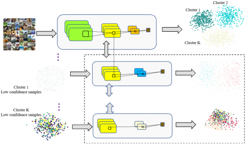
The DCNN is a tree-like deep neural network. In the network, each node classifies the data that are easy to separate early on, and determine the node of the expert network to handle the images with very slight differences (e.g., eagle image and dove image). Figure 1 illustrates the architecture of the DCNN. The network consists of N levels, each of which with K confusion clusters. The convolutional layers on different levels perform convolution at different depths.
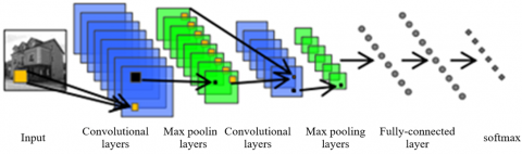
Figure 2 describes the structure of level 1 of the DCNN. After being imported to the level, the multi-class images will go through multiple convolutional layers, multiple max pooling layers, a fully-connected layer, and an output layer activated by softmax. The maximum number of max pooling layers varies from level to level.
Different from other CNN applications, our DCNN encompasses multiple convolutional layers. The learning of our network obviously requires largescale or high-level features. During image classification, the limited number of convolutional layers in the network greatly reduces the number of parameters to be learned, which helps avoid overfitting. In addition, the network training was improved and accelerated by various techniques like DropOut and batch normalization. The learning parameters of these techniques were selected based on typical values or empirical research.
Figure 1. The architecture of the DCNN
Figure 2. The structure of level 1
Based on the given dataset, level 1 of the DCNN was trained by the backpropagation algorithm [16]. The network was thus optimized to the reasonable performance. If the pre-trained network already reaches the reasonable performance, it could be directly used as a node network. Then, the confusion matrix calculated on the validation dataset was adopted to identify the cluster of each sample, such that the confusion of intra-cluster sets is much higher than that of inter-cluster sets. After network training, the data of each cluster were captured by the expert network, aiming to correct the samples that were classified incorrectly or at a low confidence.
As a result, the classification problem was zoomed in and solved as the network level deepened. The network was built up continuously until its performance on the validation dataset further improved. During the testing, the samples were classified on multiple levels of the DCNN until their classes were finalize.
There is some crux discrepancy between the architecture of the DCNN and that of traditional deep networks. First, the DCNN freezes all levels before the previous level, and trains the newly added level; these levels constitute the nodes of the next level. Second, each node is built in the feature space of the parent node and can be trained from any layer of the parent node, and the level can be selected based on the cross-validation dataset.
3.2 Data classification
The spectrum co-clustering algorithm [17] was employed to identify clusters on each node of the DCNN. This algorithm can approximate the cut of the bipartite picture (symmetric matrix) normalized to find the subgraph (sub-matrix) with significant weight, thereby realizing the block diagnosis on the matrix.
To visualize the performance of our model, the authors applied the spectral copolymerization algorithm to solve for the covariance in the confusion matrix. Thus, the diagonal in the confusion matrix is a cluster division, and these clusters are not without intersection, i.e., the clusters are not overlapping each other. In addition, the samples within the clusters can be confused. Note, however, there is an extremely low possibility of misclassification for all samples that are not on the diagonal in the confusion matrix.
To minimize the possibility of such misclassification, the joint loss, which combines softmax and WCL, was selected to finetune network parameters. The finetuning will be detailed in Subsection 3.3. To obtain the optimal number of clusters C∗, the fitness metric fm(C) was defined for the number of clusters C given by the spectrum co-clustering algorithm:
$\mathrm{fm}(\mathrm{C})=\left(\varepsilon+\frac{1}{k} \sum_{i=1}^{k}\left|C_{i}\right|\right)$ (1)
where, ε is the non-classification error caused by data splitting; Ci is the i-th cluster; |•| is the cluster size. Then the optimal number of cluster C* can be obtained as:
$C^{*}=\arg \min _{c} \mathrm{f} m(C)$ (2)
3.3 Joint loss
As mentioned before, the error caused by the inability to correctly allocate the samples to the corresponding cluster cannot be recovered. For example, suppose the level 1 subnetwork (trained with a loss function) fails to classify some images on planes, dogs, and ships. If the classes of planes and ships form a cluster, and the plane images incorrectly identified as dogs by the subnetwork are all allocated to the wrong cluster (expert node), it could not be able to assign the correct class (plane) to these graphs. In order to minimize the probability of this misclassification, the classification error was weighed to drive the contrast loss function to increase the maximum soft loss. This facilitates the block diagonalization of the confusion matrix (Figures 5 and 6). Naturally, the total loss function can be obtained as:
$L=\lambda_{2} \times L_{m}+\lambda_{1} \times L_{\text {softmax }}$ (3)
where, Lm is the WCL function. Based on the performance of the validation dataset, weights λ1 and λ2 were configured according to different image classification datasets. For example, the two weights were set to 0.8 and 1, respectively, for the MNIST experiment.
The WCL Lm can be understood as a set of soft constraints with a higher penalty for misclassification of samples to a class in another cluster than that to a class in the same cluster. That is, the similarity measure between intra-cluster samples will be smaller than that between inter-cluster samples by minimizing the WCL. The WCL function can be given by:
$L_{\mathrm{m}}=\omega_{\mathrm{ij}} \times\left(\frac{1-\delta}{2} \times \beta^{2}+\frac{\delta}{2} \times\{\max (0, m-\beta)\}^{2}\right)$ (4)
where, $\omega_{\mathrm{ij}}=\left\{\begin{array}{ll}0.1 & \text { if } i \subset C_{\mathrm{k}} \text { and } j \subset \mathrm{C}_{\mathrm{k}} \\ 1 & \text { otherwise }\end{array}\right.$ is the weight for the class labels i and j; β is the L2 norm between each pair of samples; σ is the label indicating the similarity or dissimilarity between samples; m is the margin; Ck is the kth cluster.
Our network classifies confidence samples with different number of classes, and divides the residual data that are difficult to classify into smaller clusters. Data clustering [18] makes it difficult to distinguish intra-cluster samples, but easy to differentiate between inter-cluster samples with the classified trained in the current phase [19]. Although the DCNN implicitly acquires the ability to explicitly classify samples, its robustness needs to be further improved. Therefore, the MLR was conducted on images of different classes to expand single eigenvariable into multiple eigenvariables. Through the complex calculation, the network will be more robust and accurate in image classification.
4.1 Mathematical model
Suppose variables y and x obey the following relationship:
$y=\beta_{0}+\beta_{1} x_{1}+\beta_{2} x_{2}+\cdots+\beta_{m} x_{m}+\varepsilon$ (5)
where, y is a random variable; $x_{1} ; x_{2} ; \ldots ; x_{m}$ are non-random variables; $\beta_{1} ; \beta_{2} ; \cdots ; \beta_{m}$ are regression coefficients; ε is a random error induced by various other random factors that cannot be explained by $x_{1} ; x_{2} ; \ldots ; x_{m}$ in y.
The y value in the mean E(y) must be estimated with $\beta_{0}+\beta_{1} x_{1}+\beta_{2} x_{2}+\cdots+\beta_{m} x_{m}$. This means $E(y)=\beta_{0}+\beta_{1} x_{1}+\beta_{2} x_{2}+\cdots+\beta_{m} x_{m}+\varepsilon$. Assuming that $\varepsilon \sim N\left(0, \sigma^{2}\right), y \sim N\left(\beta_{0}+\beta_{1} x_{1}+\beta_{2} x_{2}+\cdots+\beta_{m} x_{m}, \sigma^{2}\right)$, $\beta_{i}(i=0,1,2, \ldots, m)$, and that the unknown constants, $\beta_{1} ; \beta_{2} ; \cdots ; \beta_{m}$, and σ2 are not related to $x_{1} ; x_{2} ; \ldots ; x_{m}$, the n independent observation datasets obtain through the independent tests on n pairs of variables $\left(x_{1}, x_{2}, \ldots, x_{m}, y\right)$ can be expressed as:
$\left(x_{i 1}, x_{i 2}, x_{i m}, y_{i}\right), i=1,2, \ldots, n$ (6)
Moreover, the relationship between the n independent observation datasets $\left(x_{i 1}, x_{i 2}, x_{i m}, y_{i}\right),(i=1,2, \ldots, n)$ and variables $\left(x_{1}, x_{2}, \ldots, x_{m}, y\right)$ must satisfy:
$\left\{\begin{array}{c}y_{1}=\beta_{0}+\beta_{1} x_{11}+\beta_{2} x_{12}+\cdots+\beta_{m} x_{1 m}+\varepsilon_{1} \\ y_{2}=\beta_{0}+\beta_{1} x_{21}+\beta_{2} x_{22}+\cdots+\beta_{m} x_{2 m}+\varepsilon_{2} \\ \ldots \ldots \\ y_{n}=\beta_{0}+\beta_{1} x_{n 1}+\beta_{2} x_{n 2}+\cdots+\beta_{m n} x_{n m}+\varepsilon_{n}\end{array}\right.$ (7)
where, $\beta_{0}, \beta_{1}, \ldots, \beta_{m}$ are the parameters to be estimated; $\varepsilon_{1}, \varepsilon_{2}, \ldots, \varepsilon_{n}$ are n mutually independent random variables that obey normal disruption $N\left(0, \sigma^{2}\right)$. Formula (7) is the mathematical model of MLR.
Further, he MLR model (7) was constructed into the augmented Lagrangian method in the primitive dual method, aiming to speed up the convergence. Since the Lagrangian function can solve optimization problems under multiple constraints, an optimization problem with n variables and k constraints can be converted into a problem whose solution is an equation set with n+k variables. The augmented Lagrangian method is a Lagrangian method with additional penalty. By this method, the simple MLR model above was transformed into convex optimization. The Lagrangian function could be expressed as:
$L(\mathrm{x}, \lambda)=y_{n}+\lambda T(\mathrm{Ax}-b)$ (8)
The original problem is to solve $\min x f(x)$ under constraints. The new problem is solving dual problem maxλ minx L(x, λ). The optimal solutions of the two problems are equivalent, and the constraints have been removed. By the dual ascent method, we have:
step1 $: x^{k+1}=\operatorname{argmin}_{x} L\left(x ; \lambda^{k}\right)$
step2 $: \lambda^{k+1}=\lambda^{k}+\rho\left(A x^{k+1}-b\right)$ (9)
The dual ascent method splits maxλ minx L(x, λ) into two steps: solving $\min _{x} L\left(x ; \lambda^{k}\right)$ under a fixed λ; substituting the solved x into the Lagrangian function to obtain the update formula of λ through gradient descent.
To speed up the convergence, an additional penalty term was added. Then, the augmented Lagrangian function can be expressed as:
$L(x ; \lambda)=y_{n}+\lambda^{T}(A x-b)+\frac{\rho}{2}\|A x-b\|^{2}$ (10)
The ADMM was adopted to solve the Lagrangian function constructed by the MLR model. The corresponding ADMM can be defined as:
$L(x, z ; \lambda)=y_{n}+g(z)+\lambda^{T}(A x+B z-c)+\frac{\rho}{2}\|A x+B z-c\|^{2}$ (11)
Similar to the augmented Lagrangian method, two variables were fixed to update the third variable:
step1 $: x^{k+1}=\operatorname{argmin}_{x} L\left(x, z^{k}, \lambda^{k}\right)$
step2 $: z^{k+1}=\operatorname{argmin}_{z} L\left(x^{k+1}, z, \lambda^{k}\right)$
step3 $: \lambda^{k+1}=\lambda^{k}+\rho(A x+B z-c)$ (12)
Then, the problem becomes how to solve argminxL. Then, the gradient descent was adopted to solve the problem. In this way, the image features were subject to MLR, and their correlations with dimensions were clearly identified.
To verify its superiority, our method was compared with some of the most advanced algorithms, namely, stochastic pooling [20], CNN + Spearmint [21], convolutional MaxOut (COMO) + DropOut [22], network in network (NIN) + DropOut [23], and AlexNet, through experiments on a server with multiple Titan-X GPU.
5.1 Experimental results on DCNN
5.1.1 Experiment on MNIST dataset
To validate the DCNN [24], a control experiment was conducted on a subset of MNIST [25] dataset. The LeNet was taken as the starting child node of level 1. For each subsequent level (expert node), a convolutional layer and a fully-connected layer were added to deepen the classification, while only processing the subsets that are difficult to separate. From the confusion matrix generated in level 1, the numbers 3 and 5 formed a cluster (set of confusion classes). Some of the confusion samples are displayed in Figure 3. To overcome the confusion, an expert network node was established on level 2, which falls in the feature space of level 1. As shown in Figure 3, some confusion samples on level 1 were solved on level 2, indicating that the addition of level 2 improves the classification accuracy. Note that the network growth was terminated when the subsequent network could no longer distinguish or improve the validation dataset, because the generated network is data-driven.
Figure 3. The confusion samples in MNIST dataset
5.1.2 Experiment on DCNN classification
After an image was imported, the feedforward was After importing the image data, the model parameters are first optimized in DCNN by performing antecedent feedback from the root node in layer 1 and obtaining a confidence score from the function layer. If the score is higher than the threshold (obtained by pre-training), the model training is considered to have reached convergence and is used as the final output; otherwise, the image data are fed into the network branch corresponding to the other prediction labels. The whole training process is performed until the prediction score exceeds the confidence score or the image data information is transferred to the final leaf node. Finally, the response of the model can be obtained as:
$f(I)=\left\{\begin{array}{cl}\mathrm{x}_{1} & \text { if } \left.\left(\hat{I}_{s j=1}=f_{s j=1}(I)\right)\right\rangle T_{s j=1} \\ \mathrm{x}_{2} & \text { if } \left.\left(\hat{I}_{s j=2}=f_{s j=2}\left(\hat{I}_{s j=1}\right)\right)\right\rangle T_{s j=2} \\ \vdots & \vdots \\ \mathrm{x}_{\mathrm{n}} & \text { if } \left.\left(\hat{I}_{s j=n}=f_{s j=n-1}\left(\hat{I}_{s j=n-1}\right)\right)\right\rangle T_{s j=n}\end{array}\right.$ (13)
where, I is the input grapic; x is the predicted label; sj is the different phases of the network (j $\in$1, …, n; n is the number of phases); f(·) is the embedding function on each level; ^I is the output of the previous level; Tsj is the threshold for class label i in phase sj.
Further classification was made based on the confidence scores. From Table 1, it can be seen that our method outshined all advanced methods on MNIST dataset in terms of the classification performance and recognition probability of each type of number. These testify the stability of our method in image classification. For example, our method classified numbers four and nine accurately, thanks to the optimization based on confidence scores. By contrast, AlexNet, the most advanced method for image recognition and classification, failed to recognize some classes at a high accuracy, namely, numbers four and nine. The low accuracy stems from the similar classification probabilities of the two classes outputted by softmax in the network.
Table 1. The classification accuracies on MNIST dataset
|
Method |
0 |
1 |
2 |
3 |
4 |
5 |
6 |
7 |
8 |
9 |
|
Stochastic pooling [25] |
0.85 |
0.82 |
0.86 |
0.81 |
0.79 |
0.82 |
0.86 |
0.84 |
0.83 |
0.81 |
|
CNN + Spearmint [26] |
0.88 |
0.86 |
0.87 |
0.83 |
0.80 |
0.83 |
0.85 |
0.86 |
0.87 |
0.85 |
|
COMO + DropOut [5] |
0.90 |
0.92 |
0.88 |
0.87 |
0.82 |
0.88 |
0.86 |
0.89 |
0.93 |
0.91 |
|
NIN + DropOut [15] |
0.92 |
0.92 |
0.96 |
0.91 |
0.83 |
0.92 |
0.91 |
0.94 |
0.89 |
0.86 |
|
AlexNet [1] |
0.95 |
0.93 |
0.94 |
0.95 |
0.93 |
0.95 |
0.93 |
0.91 |
0.92 |
0.89 |
|
Our method |
0.97 |
0.96 |
0.97 |
0.96 |
0.98 |
0.97 |
0.95 |
0.96 |
0.95 |
0.93 |
5.2 Experimental results on MLR
Our method was compared with other state of the art methods on public benchmark datasets: CIFAR-10 and CIFAR-100. The MLR algorithm was realized on Caffe [25]. The test set was configured, and the data were preprocessed by the procedure proposed by Ioffe, S., Szegedy, C.
5.2.1 Network details
The network in Figure 2 was chosen as the root node of our DCNN. Experiments are performed on the CIFAR-10 and CIFAR-100 datasets. The child nodes can be any existing network, and all network parameter settings, weight initialization and learning strategies strictly follow the settings provided by NIN. The only exception is that the learning rate and step size were set to 0.01 and 25K, respectively, for the additional new level (shallow network).
For the two datasets, only two levels were designed: level 1 for the child node CNN, and level 2 for multiple multilayer perceptron (MLP) units. Each MLP is a cluster composed of the most confusing classes. This network structure has a very good feature: there exists a basic unit for the MLP convolutional layer, and each additional level (shallow network/branch node) is an MLP convolutional layer. The additional level was introduced after the second MLP convolutional layer to utilize the local feature response, rather than after the third node that seems to capture the specific features of the global class.
5.2.2 CIFAR-10
CIFAR-10 dataset [26] consists of 10 classes of natural images, with a total of 50K training images and a total of 10K test images. The size of each image is 32x32, and the global contrast normalization and ZCA whitening were implemented to preprocess these images. For the validation dataset, samples from the past 10K training were used to determine confidence thresholds and data segmentation based on confusion matrices [27]. After the data segmentation and confidence levels were determined, the training and validation datasets were combined to retrain the network before splitting [28].
The feature space of network learning on CIFAR-10 was visualized in Figure 4, where each point stands for an image in the dataset. The color of the point reflects the image class. It can be seen that the samples in some classes were clustered, while those in some other classes were separated. e.g., Class-1 (dark-blue) and Class-9 (yellow) were close to each other, yet far away from other classes, because they belong to the same cluster.
Figure 4. The feature space of network learning on CIFAR-10
Table 2. Classification accuracy of CIFAR-10 dataset
|
Method |
Accuracy |
|
AlexNet Stochastic pooling CNN+Spearmint COMO+DropOut NIN+DropOut |
90.23 84.89 85.02 88.34 89.58 |
|
Our method |
92.31 |
Table 2 compares the performance of our method with that of the existing methods on CIFAR dataset. Without any data enhancement, our method controlled the test error to an all-time low of 9.77% on that dataset. The performance of our method was nearly 2% better than the strong baseline method AlexNet (which has the same complexity).
5.2.3 CIFAR-100
CIFAR-100 dataset, consisting of 100 classes of natural image, is very challenging compared to the CIFAR-10 dataset. It encompasses 50K training images and 10K test images. Meanwhile, the number of training samples for CIFAR-10 is 1,000. The dataset is preprocessed using global contrast normalization and ZCA whitening, as described in the literature. Similar to NIN, the final training set of 10K samples was used as the validation dataset.
As shown in Table 3, our method had a test accuracy of 69.37%, nearly 4% better than the latest and best level achieved by AlexNet. Note that, NIN + DropOut [29] was tested after data enhancement. Even without data enhancement, our DCNN realized better performance than NIN + DropOut. This is attributable to the optimization and scheduling by the MLR.
Table 3. Classification accuracy of CIFAR-100 dataset
|
Method |
Accuracy |
|
AlexNet Stochastic pooling COMO+DropOut NIN+DropOut Learned pooling Tree based priors |
65.42 57.51 61.45 64.34 56.28 63.17 |
|
Our method |
69.37 |
5.3 DCNN performance improvement by MLR
Table 4 details the DCNN performance improvement by MLR. The DCNN was compared with the baseline method NIN. As shown in Table 4, the DCNN provided some insights into the data, such as which classes are difficult to separate. Taking CIFAR-10 for instance, three clusters of confusion classes were produced by the child node. The performance on cluster-3 was poorer than that on other clusters, because the six animal classes (cats, dogs, deer, dogs, frogs, and horses) are harder to distinguish than the classes (cars, and trucks) in cluster-2. It was also observed that the DCNN improved the performance on each cluster, thereby improving the overall performance.
This testifies that expert network node is more helpful than the end-to-end training of a large network. On CIFAR-100, the DCNN achieved a much better performance than NIN. The advantage is partly the result of the fact that the DCNN benefit more from the numerous classes in the dataset. There is still a lot of room for improvement on this particular dataset.
Table 4. The details on performance of CIFAR-10 and CIFAR-100
|
|
CIFAR-10 |
CIFAR-100 |
||||||
|
|
NIN |
Our method |
NIN |
Our method |
||||
|
|
Accuracy (%) |
Level-0 |
Level-1 |
Accuracy (%) |
Accuracy (%) |
Level-0 |
Level-1 |
Accuracy (%) |
|
Cluster-1 Cluster-2 Cluster-3 Cluster-4 Cluster-5 Cluster-6 |
92.85 94.5 77.57 - - - |
1,148 668 1,704 - - - |
767 1280 4199 - - - |
93.0 95.2 81.8 - - - |
62.03 86.0 76.0 73.65 71.38 76.0 |
1,802 102 88 548 213 89 |
5,093 0 0 983 483 0 |
65.48 86.0 76.0 76.65 73.75 76.0 |
|
Overall |
90.1 |
|
|
90.32 |
65.27 |
|
|
69.45 |
The introduction of expert network node only aims to solve clusters with at least two classes. Thus, the performance on clusters with only one class was not improved at all. This means the DCNN design will not undermine the performance of any network at the root. Instead, the DCNN only tries to improve performance by solving the most confusing situations. The clusters with at least two classes can benefit from expert network node, resulting in better overall performance.
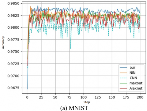
To prove the stability and robustness of our method, the accuracy and loss during training are plotted as shown in Figures 5 and 6. It was learned that our model achieved the fastest rise of accuracy in any dataset, and stabilized at the peak accuracy, albeit slight oscillations. The advantage of our model was particularly obvious on CIFAR=10, where its accuracy was 2% higher than that of the state-of-the-art NIN model. As mentioned above, our model makes better use of the data without using the domain, and the data are processed by multiple regression algorithm [30].
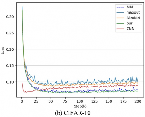
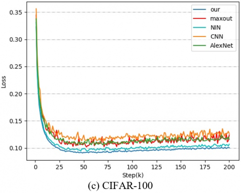
Similarly, the loss in Figure 6 indicates that our model converged quickly and tended to be stable during training. No model crash occurred due to the depth of the network, because our subsequent expert network and the antecedent network complement each other, and the best samples are chosen by multiple regression in each domain. These are the reasons for the stability and fast convergence of model training.
Figure 5. Accuracy of the training process
Figure 6. Losses of the training process
This paper proposes a general framework to build an efficient deep learning network with good classification performance on multi-class image. Our DCNN adopts a tree-like architecture, and takes CNN of different structures as child nodes (expert networks). Besides, the MLR was introduced to analyze the accuracy and robustness of the DCNN on multi-class images. Compared with the most advanced methods, our DCNN achieved excellent results on public datasets. The excellence comes from the early decisions made in the deep network [31]. Thus, the proposed method can solve any classification problem accurately in real time.
This paper was supported by Jiangsu Province Industry-University-Research Cooperation Project (Grant No.: BY2018191).
[1] Wang, Z.M., Zhang, H. (2019). A fast image retrieval method based on multi-layer CNN features. Journal of Computer-Aided Design & Computer Graphics, 31(8): 1410-1416. https://doi.org/10.3724/SP.J.1089.2019.17845
[2] Watt, N., du Plessis, M.C. (2019). Dropout for recurrent neural networks. INNS Big Data and Deep Learning Conference, Sestri Levante, Italy, pp. 38-47. https://doi.org/10.1007/978-3-030-16841-4_5
[3] Zhang, Q., Yang, L. T., Chen, Z., Li, P. (2018). A dropconnect deep computation model for highly heterogeneous data feature learning in mobile sensing networks. IEEE Network, 32(4): 22-27. https://doi.org/10.1109/MNET.2018.1700365
[4] Hamker, F.H. (2004). Predictions of a model of spatial attention using sum-and max-pooling functions. Neurocomputing, 56: 329-343. https://doi.org/10.1016/j.neucom.2003.09.006
[5] Ioffe, S., Szegedy, C. (2015). Batch normalization: accelerating deep network training by reducing internal covariate shift. arXiv preprint arXiv:1502.03167.
[6] Riquelme, C., Tucker, G., Snoek, J. (2018). Deep Bayesian bandits showdown: An empirical comparison of Bayesian deep networks for Thompson sampling. arXiv preprint arXiv:1802.09127.
[7] Feng, Y. (2015). The Analysis and Forensic Research of Heterogeneous Image. Dalian University of Technology.
[8] Huang, Q., Huang, D.H., Huang, H., Liu, Q., Xie, N.H. (2020). Recognition of incident power monitoring pattern by CNN based on AlexNet model. Radio & TV Journal, 155(3): 44-47.
[9] Zhang, L., Bi, X.J., Wang, Y.J. (2018). The ε constrained multi-objective decomposition optimization algorithm based on re-matching strategy. Acta Electronica Sinica, 46(5): 1032-1040. https://doi.org/10.3969/j.issn.0372-2112.2018.05.002
[10] Shao, B.L., He, J.N., Bian, G.Q. (2020). Research on replica layout algorithm based on multi- objective decomposition strategy. Journal of Frontiers of Computer Science and Technology, (9): 1490-1500. https://doi.org/10.3778/j.issn.1673-9418.1908062
[11] Zhang, B., Yang, Y., Lu, W.W., Wang, X.S., Xiao, S.P. (2020). A study on fully polarimetric RCS statistical characteristics of fixed-wing UAV in Ku band. Modern Radar, (6): 41-47.
[12] Song, W.Y. (2019). PolSAR Image Classification Based on Statistical Distribution and Random Field Model. Xidian University.
[13] Zhao, J.H., Liu, N. (2020). A safe semi-supervised classification algorithm based on sample selection. System Simulation Technology, 16(1): 7-11.
[14] Zhang, Y.P., Zhao, Z.J., Zheng, S.L. (2018). Spectrum handoff method by using joint optimization of cumulative delay and channel capacity based on multi-objective PSO. Telecommunications Science, 34(7): 68-77. https://doi.org/10.11959/j.issn.1000-0801.2018114
[15] Goodfellow, I., Warde-Farley, D., Mirza, M., Courville, A., Bengio, Y. (2013). Maxout networks. Proceedings of the 30th International Conference on Machine Learning, PMLR, 28(3): 1319-1327.
[16] Che, Z., Purushotham, S., Cho, K., Sontag, D., Liu, Y. (2018). Recurrent neural networks for multivariate time series with missing values. Scientific Reports, 8(1): 1-12. https://doi.org/10.1038/s41598-018-24271-9
[17] Jeong, Y., Lee, J., Moon, J., Shin, J.H., Lu, W.D. (2018). K-means data clustering with memristor networks. Nano Letters, 18(7): 4447-4453. https://doi.org/10.1021/acs.nanolett.8b01526
[18] Heisig, J.P., Schaeffer, M., Giesecke, J. (2017). The costs of simplicity: Why multilevel models may benefit from accounting for cross-cluster differences in the effects of controls. American Sociological Review, 82(4): 796-827. https://doi.org/10.1177/0003122417717901
[19] Deng, L. (2012). The mnist database of handwritten digit images for machine learning research [best of the web]. IEEE Signal Processing Magazine, 29(6): 141-142. https://doi.org/10.1109/MSP.2012.2211477
[20] Loureiro, G.B., Ferreira, J.C.E., Messerschmidt, P.H.Z. (2020). Design structure network (DSN): A method to make explicit the product design specification process for mass customization. Research in Engineering Design, 31(2): 197-220. https://doi.org/10.1007/s00163-020-00331-y
[21] Snoek, J., Larochelle, H., Adams, R.P. (2012). Practical Bayesian optimization of machine learning algorithms. Advances in Neural Information Processing Systems, 25: 2951-2959.
[22] Huang, Y., Sun, X., Lu, M., Xu, M. (2015). Channel-max, channel-drop and stochastic max-pooling. 2015 IEEE Conference on Computer Vision and Pattern Recognition Workshops (CVPRW), Boston, MA, pp. 9-17. https://doi.org/10.1109/CVPRW.2015.7301267
[23] Lin, M., Chen, Q., Yan, S. (2013). Network in network. arXiv preprint arXiv:1312.4400.
[24] Zeiler, M.D., Fergus, R. (2013). Stochastic pooling for regularization of deep convolutional neural networks. arXiv preprint arXiv:1301.3557.
[25] Delahunt, C.B., Kutz, J.N. (2019). Putting a bug in ML: The moth olfactory network learns to read MNIST. Neural Networks, 118: 54-64. https://doi.org/10.1016/j.neunet.2019.05.012
[26] Yan, Z., Zhang, H., Piramuthu, R., Jagadeesh, V., DeCoste, D., Di, W., Yu, Y. (2015). HD-CNN: hierarchical deep convolutional neural networks for large scale visual recognition. 2015 IEEE International Conference on Computer Vision (ICCV), Santiago, pp. 2740-2748. https://doi.org/10.1109/ICCV.2015.314
[27] Miyato, T., Kataoka, T., Koyama, M., Yoshida, Y. (2018). Spectral normalization for generative adversarial networks. arXiv preprint arXiv:1802.05957.
[28] Liu, Y., Liu, S., Wang, Y., Lombardi, F., Han, J. (2018). A stochastic computational multi-layer perceptron with backward propagation. IEEE Transactions on Computers, 67(9): 1273-1286. https://doi.org/10.1109/TC.2018.2817237
[29] Kessy, A., Lewin, A., Strimmer, K. (2018). Optimal whitening and decorrelation. The American Statistician, 72(4): 309-314. https://doi.org/10.1080/00031305.2016.1277159
[30] Malinowski, M., Fritz, M. (2013). Learning smooth pooling regions for visual recognition. In 24th British Machine Vision Conference, Bristol, UK, pp. 1-11. https://doi.org/10.5244/C.27.118
[31] Srivastava, N., Salakhutdinov, R.R. (2013). Discriminative transfer learning with tree-based priors. NIPS'13: Proceedings of the 26th International Conference on Neural Information Processing Systems, 2: 2094-2102.