Akram Isvand Rahmani* | Mohammad Almasi | Nastaran Saleh | Moosa Katouli
© 2020 IIETA. This article is published by IIETA and is licensed under the CC BY 4.0 license (http://creativecommons.org/licenses/by/4.0/).
OPEN ACCESS
Fusion image is the method of extracting the relevant information from two or more identical input images into one scene and creating a new image. This method allows the new image to provide comprehensive information about the wand, leading to a visual understanding of the human being. Fusion image application in image processing is an important issue. Applications in many fields such as photography, microscopy, astronomy, medical imaging, satellite imagery, machine vision, biology are monitored. In this study first, an image fusion method, suggested recently based on transform empirical wavelet, was implemented in which coefficients were obtained by processing the input images. Then they were combined by applying the rules. The aim of this study is to investigate the noise effect and to remove the noise in the aforementioned suggested method. First, the noise was added to the images, and the images were decomposed into layers or coefficients. Second, by thresholding the coefficients, the noise was removed. Then the coefficients were combined based on the rules to obtain the final coefficients. In the end, the final coefficients were used to obtain the fused image. The results show that the noise removal of images during image fusion is much better and more effective than denoising before image fusion, and the demonstration of the method is proved by obtaining better results in comparison to some existing methods.
simultaneous empirical wavelet transform, merge rules, coefficients, layers
Image fusion is the combination of two or more different images from a similar scene by an algorithm to create a new image [1]. As a result, it displays more and more relevant information.
Image fusion is used in a variety of processes, including microscopic, satellite, and medical imaging that in this article, the medical application is considered [2]. The integration of medical images is an essential process in creating an image of several different images to increase the power of diagnosis in medical discussions. The purpose of any medical information retrieval system is to provide relevant information to the appropriate user promptly. Images are of particular importance as a form of documentation that can convey a significant amount of information. One of the most important applications of images is in the field of medicine - education, research, and diagnosis, which on the one hand, due to the increasing number of medical images as a result of imaging, has become particularly important. On the other hand, recent advances in medicine, including decision-making support systems and evidence-based medicine, have multiplied the need to integrate images. CT scans, computed tomography scans, are examples of this type of imaging that are used to understand the details of an image and to integrate images [3]. Researchers have divided the methods of merging images into two categories; the transform domain and the spatial domain [4]. For example, in the field of space, we can refer to the Fast Intensity Hue Saturation (FIHS method), and in the field of transformation, we can refer to the Discrete Wavelet Transform (DWT) method that in this article the Transform domain method is considered [5].
A method [6] is proposed to integrate images based on discrete waveform conversion. In this type of conversion, the image is transferred from the spatial domain to the frequency domain. The image is first divided into horizontal and vertical components. Then the image is separated into four sections, LL1, LH1, HL1, HH1. Besides, these four sections display the four frequency zones in the image. For the low-frequency domain, LL1 is sensitive to the human eye. The problem with this method is that it decomposes the images based on predefined and fixed waves, which leads to poor image quality.
Another method that is used to analyze images is called the empirical mode decomposition (EMD) [7]. EMD is a widely used algorithm for analyzing nonlinear and non-static signals.
This method is based on the analysis of the signal to its constituent IMFs that each of them has a significant instantaneous frequency [8]. The EMD method is used in various fields, including image fusion [9]. However, the biggest drawback of this nonlinear algorithm is that it does not have a closed mathematical relationship, so we cannot predict or even estimate the output and behavior of this algorithm. In addition, EMD is a method based on sequential calculations and repetition that usually takes a long time. Sometimes we want to predict our output shape before performing the calculations. However, the EMD method does not allow us to do so under the stated conditions [10]. After this method, another method called empirical wavelet transform EWT was introduced [11].
EWT is a new way to create filters for suitable banks (similar to DWT) to extract signal-forming modes that leads us to a new violet conversion, called empirical wavelet transform. The most important difference between this conversion and EMD is that the relationship is closed, which allows us to estimate the behavior and even the overall shape of the conversion output [12].
The EWT method causes images to be thrown in different sets while being decomposed, which makes them less desirable when reconstructing images. Finally, Zhang et al. [13] provides a method called Simultaneous Empirical Wavelet Transform (SEWT) to overcome this weakness.
In this method, all input images can be decomposed into the same sets and created according to their input images. Our goal is to investigate the noise effect of noise and noise in the proposed method. The first step is to deal with adding noise to the images and dividing the images into layers or coefficients. Then, the noise is removed by applying coefficients to it. Then, after eliminating the noise, the coefficients are applied. We combine the rules to obtain the final coefficients. Ultimately, the final coefficients to get the imagined image is used. Test results show that it is a more effective method to remove the noise of images during image integration instead of deleting them.
The structure of the present manuscript is as follows: the second section presents the methodology and method of proposed method. The third section evaluates the methods examined along with the results and their comparison and analysis, and the conclusions are presented in the fourth section.
2.1 2D simultaneous empirical wavelet transform
Since in the real world, two-dimensional signals need to be processed, in the one-dimensional SEWT method, the shape of the signals was changed, and it was written to the approximate layer and the minor layers to the two-dimensional space. In such processes, some vital location information may be lost among adjacent pixels. That's why the Littlewoods-Paley two-dimensional wave converter was used [13].
Ii(p)(i=1,…….,Ni) Processed images (two-dimensional signals) with p where the pixel locations are displayed and $\mathfrak{F}_{\mathrm{P}}\left(\mathrm{I}_{\mathrm{i}}\right)(\theta,|\omega|)$ The Fourier Transform shows the polarity that "θ" refers to the Fourier Transform angle. Before identifying the February boundary for each image, it is necessary to calculate the mean spectrum with respect to "θ" such as relation (1):
$\mathscr{F}\left(I_{i}\right)(|\omega|)=\frac{1}{N_{\theta}} \sum_{k=1}^{N_{\theta}} \mathfrak{F}_{p}\left(I_{i}\right)(\theta,|\omega|)$ (1)
In relation (1), the Fourier spectrum indirectly affects the experimental Littlewoods-Paley waves. So, all the images that need to be decomposed are calculated. In relation (2), the average of the spectrum is calculated twice, according to i:
$\mathrm{F}(|\omega|)=\frac{1}{\mathrm{~N}_{\mathrm{i}}} \sum_{\mathrm{i}=1}^{\mathrm{N}_{\mathrm{i}}} \mathrm{F}\left(\mathrm{I}_{\mathrm{i}}\right)(|\omega|)=\frac{1}{\mathrm{~N}_{\mathrm{i}} \mathrm{N}_{\theta}} \sum_{\mathrm{i}=1}^{\mathrm{N}_{\mathrm{i}}} \sum_{\mathrm{i}=1}^{\mathrm{N}_{\theta}} \mathfrak{F}_{\mathrm{p}}\left(\mathrm{I}_{\mathrm{i}}\right)\left(\theta_{1},|\omega|\right)$ (2)
The mean range then identifies the Fourier boundary as in relation (2). Therefore, the diagnostic results are stored in the set, $\omega_{i}^{m}(m=1 \ldots M)$. So the set of two-dimensional simultaneous experimental wavelet transforms as that $B=\left\{\phi_{I}(p),\left\{\varphi_{m}(p)\right\}_{m=1}^{M-1}\right\},$ and $\phi_{I}(\omega)$ refers to the function of the experimental scale, and the set $\left.\left\{\varphi_{m}(t)\right\}_{m=1}^{M-1}\right\}$ shows the experimental wave transform function. Finally, the approximation layer of $\mathrm{I}_{i}(\mathrm{p})$ is defined as the relation (3):
$\mathrm{W}\left(\mathrm{I}_{\mathrm{i}}\right)(0, \mathrm{p})=\mathfrak{F}_{\omega}^{-1}\left(\mathfrak{F}_{\mathrm{p}}\left(\mathrm{f}_{\mathrm{i}}\right)(\omega) \overline{\mathscr{F}_{\mathrm{P}}\left(\phi_{1}\right)(\omega)}\right)$ (3)
The detail layers of image Ii(p) are defined as relation (4):
$\mathrm{W}\left(\mathrm{I}_{\mathrm{i}}\right)(\mathrm{m}, \mathrm{p})=\mathfrak{F}_{\mathrm{p}}^{-1}\left(\mathscr{F}_{\mathrm{p}}\left(\mathrm{I}_{\mathrm{i}}\right)(\omega) \overline{\left.\mathscr{F}_{\mathrm{P}}\left(\varphi_{\mathrm{m}}\right)(\omega)\right)}\right.$ (4)
Finally, the inverse of the two-dimensional simultaneous Empirical Wavelet Transform is defined by Eq. (5):
$\mathrm{I}_{\mathrm{i}}(\mathrm{p})=\mathrm{W}\left(\mathrm{I}_{\mathrm{i}}\right)(0, \mathrm{p}) \diamond\left(\phi_{1}\right)(\mathrm{p})+\sum_{\mathrm{m}=1}^{\mathrm{M}-1} \mathrm{~W}\left(\mathrm{I}_{\mathrm{i}}\right)(\mathrm{m}, \mathrm{p}) \diamond \varphi_{\mathrm{m}}(\mathrm{p})$ (5)
2.2 Image fusion algorithm
IA and IB show the input images with the size of M×N, and IF shows the output or fusion image [13]. The process of fusion images is done in three steps:
(1) According to the two input images IA and IB, the Simultaneous Empirical Wavelets is simultaneously created as $\mathrm{B}=\left\{\phi_{1}(\mathrm{p}),\left\{\varphi_{i}(\mathrm{p})\right\} \begin{array}{l}L-1 \\ i=1\end{array}\right\}$. These two images are then decomposed into sub-bands by using Eq. (3) and Eq. (4), $W_{A}=\left\{W_{A}^{0}, W_{A}^{1}, \ldots, W_{A}^{L}\right\} \quad$ and $\quad W_{B}=\left\{W_{B}^{0}, W_{B}^{1}, \ldots, W_{B}^{L}\right\}$ respectively.
$\mathrm{W}_{*}^{0}$ represents the approximation layer and $\mathrm{W}_{*}^{1}, \ldots, \mathrm{W}_{*}^{\mathrm{L}}$ represents the details layers.
(2) According to the designed rules, the approximation layer and details layers are combined to obtain the fused layers $\mathrm{W}_{F}=\left\{\mathrm{W}_{F}^{1}, \mathrm{~W}_{\mathrm{F}}^{1}, \ldots, \mathrm{W}_{F}^{\mathrm{L}}\right\}$. Also, $\mathrm{r}=\left\{r_{0}\left\{r_{i}\right\}_{i=1}^{L}\right\}$ shows the fusion map set, in which $r_{0}$ is fusion map for approximation layer, and $\left\{r_{i}\right\}_{i=1}^{L}$ are fusion map for detail layers.
$W_{F}^{0}=r_{0} W_{A}^{0}+\left(1-r_{0}\right) W_{R}^{0}$ (6)
and
$W_{F}^{i}=r_{i} W_{A}^{i}+\left(1-r_{i}\right) W_{B}^{i} \quad(\mathrm{i}=1, \ldots \mathrm{L})$ (7)
(3) Conducts inverse 2D SEWT on $\mathrm{W}_{F}$. This is done to obtain the merged image using relation (5) [9].
2.3 Fusion rules
For each input image in the approximation layer, relation (8) is used [13].
$\mathcal{S}\left(\mathrm{W}_{*}^{0}(\mathrm{p})\right)=\frac{1}{\mathrm{M} \times \mathrm{N}} \sum_{\mathrm{w}_{(\mathrm{q}) \square \mathrm{W}_{*}^{0}}} \mathrm{D}\left(\mathrm{W}_{*}^{0}(\mathrm{p}), \mathrm{W}_{*}^{0}(\mathrm{q})\right)$ (8)
where, $\mathrm{D}\left(\mathrm{W}_{*}^{0}(\mathrm{p}), \mathrm{W}_{*}^{0}(\mathrm{q})\right)$ indicates the distance between the intensities of the coefficients P and Q, $\mathrm{D}\left(\mathrm{W}_{*}^{0}(\mathrm{p}), \mathrm{W}_{*}^{0}(\mathrm{q})\right)=\left|\mathrm{W}_{*}^{0}(\mathrm{p})-\mathrm{W}_{*}^{0}(\mathrm{q})\right|$. According to the sigmoid function, approximation layer rule is stated:
$\mathrm{r}_{0}=\frac{1}{1+\mathrm{e}^{-\mathrm{a}\left(\mathcal{S}\left(\mathrm{w}_{\mathrm{A}}^{0}\right)-\mathcal{S}\left(\mathrm{w}_{\mathrm{B}}^{0}\right)\right)}}$ (9)
In which a is set to 0.5. The fusion rule is defined for detail layers by Eq. (10) as,
$r_{i}=\left\{\begin{array}{l}1\left|W_{A}^{i}\right|>\left|W_{A}^{i}\right| \\ 0 \text { otherwise }\end{array} \quad(i=1, \ldots . L)\right.$ (10)
In the final step, the approximation layer and the partial layers are obtained using Eq. (6) and Eq. (7) [13].
2.4 Denoising proposed
In digital image processing, de-noising technique is used to reduce, or if possible remove, noise without losing detail. There are various techniques for de-noising digital images. Gaussian noise can be reduced using a spatial filter. While smoothing an image, the blurring of fine-scaled image edges and details are possible for corresponding to the high frequencies blocked by the process [14, 15]. Among the spatial filtering techniques, the most prevalent noise removal techniques are comprised of mean (convolution) filtering, median filtering and Gaussian smoothing. Most of the standard de-noising algorithms are dealt with an individual filtering process [16]. The result decreases the noise, but the image is blurred or smoothed at lines and edges due to high frequency losses [17, 18].
In order to effectively reduce the noise together with minimum adverse outcome, this research is developed to examine and evaluate various filters and wavelet transform for analyzing a digital image in useful sub-bands. Wavelet transform and filtering, as well as a median filter are individually used for image de-noising in various domains [14]. In this work, we explore some combinations, which have the ability to produce better outcomes for digital image de-noising.
Application of empirical Wavelet Transform (DWT) approach is highlighted for digital image de-noising in the following six steps.
(1) Apply EWT on a noisy image to Divide into four sub-bands (A, H, V, D) by using wavelet filter families [14].
(2) Choose one of the suitable threshold rule methods to compute a threshold value for one of the detail bands H, V, D.
(3) Implement a comparison between pixels in the sub-bands (H, V, D) and specific threshold value for that band. Set the pixel to zero if its value is less than the threshold of the band. Otherwise, test the next pixel value. This process is repeated for all of the pixels in the selected sub-band.
(4) The inverse EWT (IEWT) is used for selected substrates to obtain a noise-free image.
(5) Apply median filter within WT alone. It is done either before or after threshold as needed in each case. The median filter is applied to the entire image using a 3x3 mask filter. Sort all of the pixel values from surrounding neighborhood in an ascending manner. Exchange the pixel to the centeral pixel value [14].
(6) implement a comparison between the de-noised and original image. It is accomplished by computing image quality for the denoising technique.
Thresholding is a simple and effective method for image segmentation, which is used for generating digital images from a grayscale image. As such, threshold technique is utilized for digital image de-noising in a beneficial manner. In this study, the threshold technique is used in digital wavelet domain. Because the conversion of the experimental waveform decomposes the images into details layers and the approximation layer, the details layers with different scales and resolutions are examined. The details layers have a higher frequency, and noise can be eliminated by different methods of thresholding.
With developing this method, the noise, from the image of the loss of vital information, should be significantly reduced, which is of interest to medical [14]. Therefore, a good threshold value would lead to less image distortion. Threshold value is computed by applying Eq. (11) as follows:
$\mathrm{Th}=\frac{\sigma^{2}}{\sigma_{x}}$ (11)
where, $\sigma^{2}$ is related to noise value of noisy image. It is computed by Robust Median Estimator, which is estimated from HH sub-band. It is defined by Eq. (12).
$\sigma^{2}=\left[\frac{\operatorname{median} \mid\left\{\mathrm{x}_{i, j}: \mathrm{i}, \mathrm{j} \in \mathrm{HH}_{1}\right\}}{0.6745}\right]^{2}$ (12)
and $\sigma_{x}$ refers to standard deviation (STD) of the sub-bands. It is computed by Eq. (13).
$\sigma=\sqrt{\frac{\sum_{i=0}^{n-1}\left(x_{i}-m\right)^{2}}{n}}$ (13)
where:
σ: standard deviation (STD),
m: mean,
n: Indicates the number of pixels in each sub-band,
xi: Indicates each sub-band.
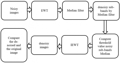
Figure 1. Denoising proposed
In the proposed denoising technique, EWT is applied on a noisy image to obtain detail sub-bands. Then, median filter is applied on each sub-band independently using Eq. (11), (12) and (13). Then, IEWT is considered for the sub-bands to obtain a de-noisy (de-noised) image. Figure 1 shows the block diagram for the third case and Median filter before threshold.
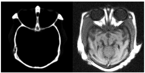
Today, medical imaging plays an essential role in clinical diagnosis and treatment. CT images, for example, are widely used in fractures because they can record bone condition. MRI scans can be used to diagnose brain diseases such as brain tumors and the like. CBF (Cerebral Blood Flow) images can objectively reflect changes in the tension and tension of cerebral arteries. SPECT images can measure the biological activity of cells and molecules. However, these images have limitations that may limit their use in real applications. Single-photon emission computed tomography (SPECT) images, for example, cannot be clear enough to absorb brain structures. Therefore, SPECT images are always used with computed tomography (CT) or MRI images for clinical diagnosis. Finally Medical images (http://www.med.harvard.edu/AANLIB/home.html) were captured by the SEWT method [13].
Also, in order to demonstrate the proposed method, some experimental results are elaborated in this section. The computer that has been used has the following specifications: Windows 8, 64-bit, Intel Core i7-4720 CPU @ 2.60 GHz, 8 GB memory, and MATLAB R2018a.
At the following, the proposed fusion method of denoising SEWT is compared with other methods, Discrete wavelet transform based algorithm (DWT) [19], Guided filtering based fusion algorithm (GFF) [2], as well as the algorithm Liu et al. (LIU) [3], Nonsubsampled contourlet transform based algorithm (NSCT) [1] and a DCT based Laplacian Pyramid (DCTLPIF) [4].
At the end, for a quantitative comparison of the proposed noise elimination algorithm, the proposed algorithm is tested on several pairs of medical images and the results are compared with some existing methods. In this study, five criteria, $Q_{\mathrm{AB}}^{\mathrm{F}}$, MI, VIFF, PSNR, and MSE, have been selected to compare algorithms. $Q_{\mathrm{AB}}^{\mathrm{F}}$ Expressive edge information is integrated from the input images to the fused image. MI Indicates the amount of information of input images to the output image. Peak-Signal-to-Noise ratio (PSNR) and Mean Square Error (MSE) express improved image quality [20].
3.1 Experiments on multi-modal medical images
In Figure 2, examples of such images are shown as input images. There are four images in each row, with the first two images being the same as the input images and the second two images being noisy images with a standard deviation value of 10.
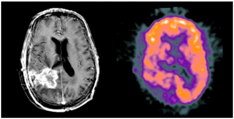
Now, to confirm the superiority of the proposed method, it has been compared with other methods in Figure 3.
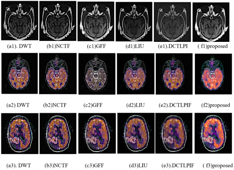
As shown in Figure 3(a1) to (f3), denoising SEWT are compared with the other five methods, and all but the first row contains color images. In fused color images, visual information must be preserved, in addition to preventing any color distortion, which is involved in methods such as images b and c. Also, the c and e images have a more pronounced mode, which weakens their performance, and it makes it difficult to see the details.
However, in the proposed method, despite the elimination of noise, the soft texture and color information are still well preserved.
Now in Table 1, we compare the denoising SEWT with other methods in terms of five quantitative criteria.
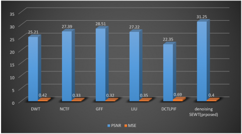
As shown in Figure 4, despite the denoising, the PSNR and MSE criteria have higher values and the less error rate.
As shown in Table 1, the three criteria for merging the proposed method images are better than the other methods. The performance of PSNR and MSE is shown with sigma=15 in Figure 4.
(a). Input images
(b). Noisy images with $\sigma=10$
(c). Input images
(d). Noisy images with $\sigma=10$
(e). Input images
(f). Noisy images with $\sigma=10$
Figure 2. Input images and noise images
3.2 Experiments on VISIBLE-IR images
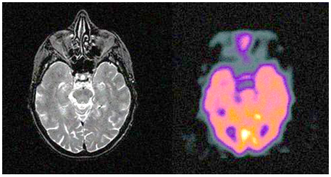
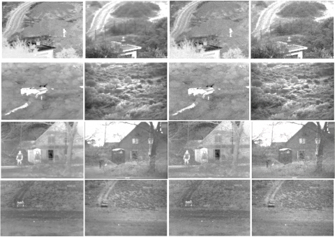
In the real world, visual images and infrared images are always integrated into one image. Visual images can only capture surface information, while infrared images can reflect internal information based on temperature. The integration of infrared and visible images allows us to improve the detection and identification of the part of the target in the infrared image, according to its background in the visual images. Figure 5 shows visible and infrared images, while the first two images in each row represent the primary images, and the second two images show the noisy images.
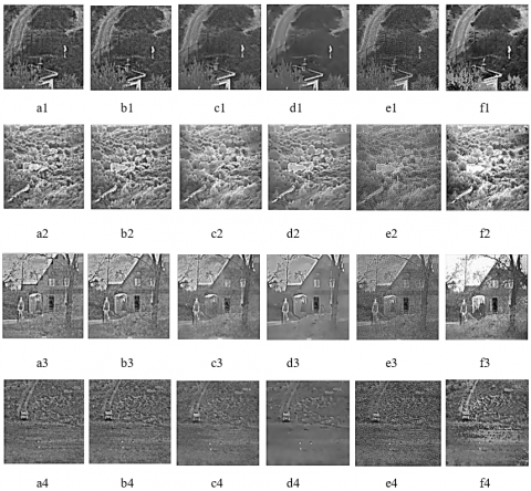
Also, From Figure 6(a1) to (f3), we list six groups of color fused denoised images.
Figure 6 shows the output images of the proposed method with other methods.
Despite the noise deletion in Figure 6(f3), In the proposed method, i.e., denoising SEWT final images, it can show more comprehensive and appropriate information than other methods. This case does not happen when we employ other methods. However, the final image loses when it is fused by other methods. It is due to the noise deletional, which makes some details invisible. Table 2 examines the quantitative criteria of the proposed method with other methods.
According to the results of the Table 2, it can be concluded that $Q_{\mathrm{AB}}^{\mathrm{F}}$ has a lower amount in the proposed method. We lose some detail information for the sake of high noise. Figure 7 shows the performance of PSNR and MSE for $\sigma=15$.
According to Figure 7, the proposed method performs better than other methods, while in the same method as GFF, it is in the second place. Other methods, such as LIU, are third, and NTCF is fourth. The DWT and DCTLPIF methods are in the next ranks, respectively.
In summary, according to Figures 3 and 7, when noise-free input images in both medical and infrared images, are combined (σ = 0), this criterion is superior to that of other methods. Nevertheless, when input images contain high amounts of noise (by applying large values of standard deviation), a great amount of the edge information is lost due to denoising by applying soft thresholding (due to its property) on the coefficients during image decomposition. This causes the merged image to be more blurred and a small amount of the edge information is lost. However, except for the LIU method, other methods have not addressed denoising during image merging process.
Figure 3. Fused denoised medical images obtained by different algorithms
Figure 4. Comparison of denoise performance of the proposed method with the other methods with sigma=15
Table 1. Average percentage of performance measurements for the proposed denoising method with respect to different Standard deviations on multi-modal medical images
|
Standard deviation |
Evaluation criterion |
a |
b |
c |
d |
e |
f |
|
$\sigma=0$ |
VIFF |
0.5528 |
0.5930 |
0.0716 |
0.4803 |
0.5105 |
0.6735 |
|
MI |
0.2484 |
0.2594 |
0.3496 |
0.2851 |
0.2818 |
0.3589 |
|
|
$Q_{A B}^{F}$ |
0.6205 |
0.6707 |
0.7569 |
0.6527 |
0.0669 |
0.7135 |
|
|
PSNR |
26.21 |
30.29 |
30.91 |
29.52 |
24.30 |
35.25 |
|
|
MSE |
0.41 |
0.30 |
0.29 |
0.31 |
0.59 |
0.21 |
|
|
$\sigma=5$ |
VIFF |
0.5476 |
0.5883 |
0.0388 |
0.4814 |
0.5273 |
0.5947 |
|
MI |
0.2196 |
0.2342 |
0.3164 |
0.2823 |
0.2920 |
0.3971 |
|
|
$Q_{A B}^{F}$ |
0.5847 |
0.6357 |
0.7332 |
0.6308 |
0.0493 |
0.6263 |
|
|
PSNR |
27.42 |
31.58 |
31.45 |
30.12 |
25.25 |
34.15 |
|
|
MSE |
0.51 |
0.42 |
0.31 |
0.45 |
0.64 |
0.27 |
|
|
$\sigma=10$ |
VIFF |
0.5174 |
0.5595 |
0.0225 |
0.4765 |
0.5151 |
0.5565 |
|
MI |
0.2071 |
0.3241 |
0.2971 |
0.2578 |
0.3010 |
0.4063 |
|
|
$Q_{A B}^{F}$ |
0.5416 |
0.5944 |
0.6745 |
0.5419 |
0.0093 |
0.5641 |
|
|
PSNR |
26.32 |
29.49 |
28.99 |
29.66 |
27.30 |
32.25 |
|
|
MSE |
0.51 |
0.32 |
0.31 |
0.32 |
0.66 |
0.32 |
|
|
$\sigma=15$ |
VIFF |
0.4725 |
0.5230 |
0.0192 |
0.4951 |
0.4521 |
0.5211 |
|
MI |
0.2189 |
0.1968 |
0.2169 |
0.2856 |
0.3664 |
0.4097 |
|
|
$Q_{A B}^{F}$ |
0.5054 |
0.5569 |
0.6415 |
0.4545 |
0.0035 |
0.5206 |
|
|
PSNR |
25.21 |
27.39 |
28.51 |
27.22 |
22.35 |
31.25 |
|
|
MSE |
0.42 |
0.33 |
0.32 |
0.35 |
0.69 |
0.40 |
Table 2. Average percentage of performance measurements for the proposed denoising method with respect to different Standard deviations on fused Visible-IR images
|
Standard deviation |
Evaluation criterion |
a |
b |
c |
d |
e |
f |
|
$\sigma=0$ |
VIFF |
0.5422 |
0.5836 |
0.0617 |
0.4719 |
0.5266 |
0.6621 |
|
MI |
0.2312 |
0.2616 |
0.3399 |
0.2844 |
0.2789 |
0.3499 |
|
|
$Q_{A B}^{F}$ |
0.6122 |
0.6614 |
0.7469 |
0.6441 |
0.0665 |
0.7078 |
|
|
PSNR |
29.52 |
30.33 |
30.42 |
29.77 |
22.96 |
33.45 |
|
|
MSE |
0.45 |
0.30 |
0.31 |
0.34 |
0.62 |
0.24 |
|
|
$\sigma=5$ |
VIFF |
0.5316 |
0.5789 |
0.0245 |
0.4712 |
0.5166 |
0.5847 |
|
MI |
0.2236 |
0.2455 |
0.3079 |
0.2911 |
0.2879 |
0.3846 |
|
|
$Q_{A B}^{F}$ |
0.5778 |
0.6243 |
0.7012 |
0.6200 |
0.0564 |
0.7089 |
|
|
PSNR |
28.44 |
31.26 |
29.90 |
30.15 |
23.330 |
34.78 |
|
|
MSE |
0.45 |
0.40 |
0.35 |
0.40 |
0.65 |
0.26 |
|
|
$\sigma=10$ |
VIFF |
0.5033 |
0.5478 |
0.0221 |
0.4600 |
0.5172 |
0.5533 |
|
MI |
0.3014 |
0.3345 |
0.2866 |
0.2478 |
0.3125 |
0.4175 |
|
|
$Q_{A B}^{F}$ |
0.5314 |
0.5879 |
0.6699 |
0.5327 |
0.009 |
0.5547 |
|
|
PSNR |
27.40 |
29.60 |
29.45 |
29.30 |
21.31 |
33.20 |
|
|
MSE |
0.52 |
0.32 |
0.37 |
0.38 |
0.70 |
0.30 |
|
|
$\sigma=15$ |
VIFF |
0.4822 |
0.5133 |
0.0189 |
0.4876 |
0.4423 |
0.5147 |
|
MI |
0.2236 |
0.1889 |
0.2056 |
0.2578 |
0.6441 |
0.4078 |
|
|
$Q_{A B}^{F}$ |
0.5011 |
0.5289 |
0.6322 |
0.4725 |
0.0036 |
0.5147 |
|
|
PSNR |
25.96 |
28.13 |
29.88 |
29.34 |
21.87 |
31.02 |
|
|
MSE |
0.42 |
0.37 |
0.32 |
0.35 |
0.74 |
0.34 |
Figure 5. Visible-IR input images and noisy images
Figure 6. Fused visible-IR images obtained by different algorithms
Figure 7. Comparison of denoise performance of the proposed method with the other methods for visible-IR images with sigma=15
This study is first dealt with implementing an image fusion method, which has recently been suggested based on transform empirical wavelet. In this research, coefficients are obtained by processing input images. Then, they are combined by applying rules. The aim of the proposed method is to investigate the amount of noise during the implementation of the image integration algorithm. In the first step, after adding noise to images, they were decomposed into layers or coefficients. In the second step, the noise was removed by thresholding the coefficients. Then, the coefficients were combined based on rules to obtain final coefficients. Ultimately, the final coefficients were used to obtain a fused image. The results showed that it is much better and more effective to remove the noise of images during image fusion than denoising before image fusion. Because of in the merging process after the image decomposition, since applying the thresholding on the coefficients is realized in the frequency domain, better image denoising is obtained than in the space domain.
Also, proposed method provided better results in comparison with some other methods. Despite the removal of noise, the amount of information transferred from the input images to the merged image was still higher, but in terms of edge information, we lose a little bit of information when removing noise, and of course, this is quite normal in the noise removal process. In future researches, Various denoising methods can be considered on the images so that the details of the images are increased, and we have enough edge information when removing the noise.
[1] Zhang, Q., Guo, B.L. (2009). Multifocus image fusion using the nonsubsampled contourlet transform. Signal Processing, 89(7): 1334-1346. https://doi.org/10.1016/j.sigpro.2009.01.012
[2] Li, S.T., Kang, X., Hu, J. (2013). Image fusion with guided filtering. IEEE Transactions on Image Processing, 22(7): 2864-2875. https://doi.org/10.1109/TIP.2013.2244222
[3] Liu, Y., Wang, Z. (2014). Simultaneous image fusion and denoising with adaptive sparse representation. IET Image Processing, 9(5): 347-357. https://doi.org/10.1049/iet-ipr.2014.0311
[4] Naidu, V.P.S. (2013). Novel image fusion techniques using DCT. International Journal of Computer Science and Business Informatics, 5(1): 1-18.
[5] Mishra, D., Palkar, B. (2015). Image fusion techniques: a review. International Journal of Computer Applications, 130(9): 7-13. https://doi.org/10.5120/ijca2015907084.
[6] Amin-Naji, M., Aghagolzadeh, A. (2018). Multi-focus image fusion in DCT domain using variance and energy of Laplacian and correlation coefficient for visual sensor networks. Journal of AI and Data Mining, 6(2): 233-250. https://doi.org/10.22044/JADM.2017.5169.1624
[7] Huang, N.E., Shen, Z., Long, S.R., Wu, M.C., Shih, H.H., Zheng, Q., Yen, N.C., Tung, C.C., Liu, H.H. (1998). The empirical mode decomposition and the Hilbert spectrum for nonlinear and non-stationary time series analysis. Proceedings of the Royal Society of London. Series A: Mathematical, Physical and Engineering Sciences, 454(1971): 903-995. https://doi.org/10.1098/rspa.1998.0193
[8] Rani, K., Sharma, R. (2013). Study of different image fusion algorithm. International Journal of Emerging Technology and Advanced Engineering, 3(5): 288-291.
[9] Hariharan, H., Gribok, A., Abidi, M.A., Koschan, A. (2006). Image fusion and enhancement via empirical mode decomposition. Journal of Pattern Recognition Research, 1(1): 16-32. https://doi.org/10.13176/11.6
[10] Looney, D., Mandic, D.P. (2009). Multiscale image fusion using complex extensions of EMD. IEEE Transactions on Signal Processing, 57(4): 1626-1630. https://doi.org/10.1109/TSP.2008.2011836
[11] Gilles, J. (2013). Empirical wavelet transform. IEEE Transactions on Signal Processing, 61(16): 3999-4010. https://doi.org/10.1109/TSP.2013.2265222
[12] Gilles, J., Tran, G., Osher, S. (2014). 2D empirical transforms. Wavelets, ridgelets, and curvelets revisited. SIAM Journal on Imaging Sciences, 7(1): 157-186. https://doi.org/10.1137/130923774
[13] Zhang, X., Li, X., Feng, Y. (2017). Image fusion based on simultaneous empirical wavelet transform. Multimedia Tools and Applications, 76(6): 8175-8193. https://doi.org/10.1007/s11042-016-3453-8
[14] Ramadhan, A., Mahmood, F., Elci, A. (2017). Image denoising by median filter in wavelet domain. arXiv preprint arXiv: 1703.06499. https://doi.org/10.5121/ijma.2017.9104
[15] Donoho, D.L. (1995). De-noising by soft-thresholding. IEEE Transactions on Information Theory, 41(3): 613-627. https://doi.org/10.1109/18.382009
[16] Donoho, D.L., Johnstone, I.M. (1995). Adapting to unknown smoothness via wavelet shrinkage. Journal of the American Statistical Association, 90(432): 1200-1224. https://doi.org/10.2307/2291512
[17] Zhang, X.P. (2001). Thresholding neural network for adaptive noise reduction. IEEE Transactions on Neural Networks, 12(3): 567-584. https://doi.org/10.1109/72.925559
[18] Donoho, D.L., Johnstone, J.M. (1994). Ideal spatial adaptation by wavelet shrinkage. Biometrika, 81(3): 425-455. https://doi.org/10.2307/2337118
[19] Helonde, M.R.P., Joshi, M.R. (2015). Image fusion based on medical images using DWT and PCA methods. International Journal of Computer Techniques, 2(1): 75-79.
[20] Zhu, Y.L., Xu, C.G., Xiao, D.G. (2019). Denoising ultrasonic echo signals with generalized s transform and singular value decomposition. Traitement du Signal, 36(2): 139-145. https://doi.org/10.18280/ts.360203