Xiaodong Yan | Xiaogang Song*
© 2020 IIETA. This article is published by IIETA and is licensed under the CC BY 4.0 license (http://creativecommons.org/licenses/by/4.0/).
OPEN ACCESS
This paper mainly designs an image recognition algorithm of bolt loss in underground pipelines. Firstly, the local binary pattern (LBP) operator was improved to optimize the information content of eigenvectors and enhance the discriminability. Next, the patterns were selected through weighting and ranking, thereby optimizing the original features in each channel of the image. Meanwhile, the main patterns of each channel were classified and identified with the support vector machine (SVM) classifier. The radial basis function (RBF) was taken as the kernel function for the SVM, and the teaching-learning-based optimization (TLBO) algorithm was improved to optimize the SVM parameters. Finally, the improved SVM classifier assigns suitable weights to the predicted class tags of different channels, facilitating the recognition of bolt loss. The research results shed new light on the application of swarm intelligence in image recognition.
image recognition, local binary pattern (LBP) operator, feature extraction, support vector machine (SVM), underground pipelines
In modern cities, an important aspect of urban planning is the construction of underground pipelines. However, the underground conditions in urban areas are very complex, and the available underground space is extremely limited. It is difficult to detect the damages of underground pipelines or the loss of relevant accessories in time.
At present, the damages of underground pipelines are mainly detected in two stages: the image of the target pipeline is captured by a robot, and then evaluated by professional inspectors. By this strategy, lots of pipeline images need to be analyzed manually, which limits the accuracy and timeliness of detection. To overcome the defects, this paper proposes an image detection algorithm of bolt loss in underground pipelines. Using image recognition technology, the proposed algorithm can automatically detect the missing position of bolts on the target pipeline.
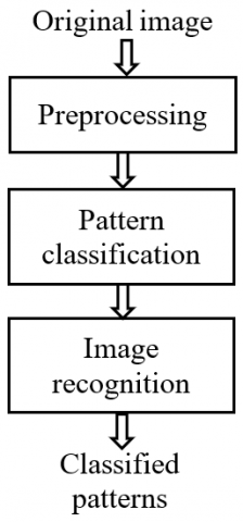
Image recognition technology [1] replaces humans with computers to process and recognize such signals as words and images, and complete the tasks of classification and identification. This technology features advanced intelligence similar to human vision. Figure 1 provides the basic flow of image recognition.
As shown in Figure 1, image recognition covers three critical steps: preprocessing, feature extraction, and pattern classification. Specifically, preprocessing filters and reduces the noise and interference signal from the original image, and transforms the brightness or color of the image, improving its visual quality and effect. Feature extraction mainly segments the region of interest (ROI), extracts the features or special information, and identifies the key features that are most conducive to classification. Pattern classification selects a suitable classifier to determine the class of the image, according to the key features. Therefore, this paper attempts to improve the image recognition performance of the proposed algorithm from the three aspects of preprocessing, feature extraction, and pattern classification.
Figure 1. The basic flow of image recognition
Under the effects of external factors and equipment conditions, the images of underground pipelines are often affected by impulse noise during the process of formation, transmission, reception, and processing. The original images usually contain various types of noises, such as Gaussian noise and salt-and-pepper noise. The negative effects of the noises are generally eliminated through filtering.
So far, many algorithms have been improved to reduce the noises in images for different applications. For example, Chen et al. [2] identified salt-and-pepper noise of the target image by grayscale difference and extreme value distribution in the local direction, and removed the identified noise through recursive or non-recursive weighted grayscale average filtering. Under the tolerance mechanism, Du [3] designed an anisotropic Gaussian filtering algorithm to protect and smoothen the edges of the target image, which successfully produces a fog-free image. Schmeing and Jiang [4] proposed a maximum median filtering algorithm that preserves the edge textures of the target image, while removing the noises. Zhu et al. [5] analyzed the statistical features of the target image in the wavelet domain, improved the wavelet function through Bayesian method, and denoised the image through wavelet thresholding and bilateral filtering; their approach effectively filters out speckle noise, and achieves a good effect of edge preservation.
Feature extraction is one of the premises of image recognition. The recognized target is usually converted into an eigenvector with low-dimensional classification information, laying the basis for subsequent pattern classification. The local binary pattern (LBP) [6] is a widely accepted descriptor of texture features. Many scholars have improved the robustness of the descriptor by optimizing the encoding method. For instance, Prakash and Prasad [7] derived the local ternary pattern (LTP) operator from differential positive and negative signs. Guo et al. [8] added amplitude into encoding, creating the compound LBP (CLBP) operator. Yang and Chen [9] proposed the centralized binary pattern (CBP) by comparing the threshold with local neighborhood mean. Considering the grayscale change of centrosymmetric pixels, Yuan et al. [10] designed the centrosymmetric LBP (CSLBP) operator. Zhu et al. [11] created the orthogonal combination of LBP (OCLBP) operator, drawing on the grayscale change of orthogonally distributed pixels. Datta Rakshit et al. [12] put forward the extended center-symmetric LBP (XCSLBP) operator, according to the grayscale change of the central pixel and the symmetrically distributed pixels.
Pattern classification identifies the classes of the target image against the judgement criteria formulated based on the eigenvectors, which are obtained in feature extraction. In the field of image classification, the most popular pattern classifiers include Bayesian classifier, decision tree (DT) classifier, nearest neighbor classifier, neural network (NN) classifier, and support vector machine (SVM) classifier [13-15]. Among them, the SVM takes root in statistical learning, and boasts excellent generalization ability. In practical application, however, the SVM parameters are selected empirically, due to the lack of theoretical basis for parameter selection. Many researchers have attempted to optimize the SVM parameters with intelligent optimization algorithms. Mo and Zhao [16] evaluated the influence of penalty factor and kernel parameters on SVM classification performance. Through particle swarm optimization (PSO), Wang et al. [17] optimized the allocation of penalty factor and kernel parameters of SVM classifier. Montiel [18] introduced the hybrid quantum genetic algorithm to optimize the parameters and enhance the accuracy of the SVM.
Feature extraction is a prerequisite for image recognition. In the field of image recognition, the LBP-based extraction of texture features is a research hotspot. However, the existing LBP operators need to be further improved. In this section, the encoding and pattern selection method of LBP operator are improved to extract eigenvectors with strong discriminability, and eliminate the interference of useless patterns.
3.1 Theory on LBP operator
The LBP operator is a feature extractor that describes the texture distribution in the local region. Taking the grayscale of the central pixel in the local region as the benchmark, the LBP operator differentiates the other pixels in the local region, encodes the direction of the local difference, statistically analyzes the codes, and extracts the local texture features of the image.
In general, the LBP operator adopts the 3×3 neighborhood centering on the current pixel as the template for encoding, and the grayscale of the current central pixel as the threshold. Along the specified direction, the central pixel is compared with the eight pixels in its neighborhood in turn. The comparison results are binarized and assigned different weights. Finally, the cumulative value of the coding is added up with the LBP code value of the current pixel. Through point-wise scanning of the entire image, an LBP response image can be obtained. The histogram of this image is called the LBP feature.
To adapt to the texture feature analysis with different image sizes and sampling intensities, Ojala et al. [19] extended the 3×3 neighborhood to a circular neighborhood with different radii and number of sampling points. In this way, the LBP operator is modified into LBPC,R:
$L B P_{C, R}=\sum_{i=0}^{C-1} u\left(g_{i}-g_{o}\right) 2^{i}$ (1)
where, go is the grayscale of the central pixel in the neighborhood; gi is the grayscale of C sampling points evenly distributed on the circle with $g_{o}$ as the center and R as the radius; u(gi-go)=1 if $g_{i} \geq g_{o}$, and u(gi-go)=0 if otherwise; 2i is the weight of each sampling point in the neighborhood, which ensures the uniqueness of LBPC,R encoding of the current go.
By the definition of LBPC,R, the C pixels in the local neighborhood can form 2C different outputs. For a region of ordinary size, the LBP operator can generate various patterns, making the final histogram so sparse as to be statistically insignificant. Pattern selection is necessary to reduce the pattern redundancy of the LBP operator, without sacrificing the ability of texture description.
For the circular neighborhood, as long as the value of u(gi-go) is not all 0 or 1, the code value of the LBP will change with the rotation angle of the image. As the circular neighborhood rotates about the current pixel, a series of different LBP code values can be obtained, of which the minimum is taken as the final LBP code of the current pixel:
$L B P_{C, R}^{t^{i}}=\min \left\{f_{R O}\left(L B P_{C, R}, i\right), i=0, \ldots, C-1\right\}$ (2)
where, fRO() is the rotation function, by which the neighborhood pixels of the current LBP operator rotates clockwise for i times.
It can be inferred from the encoding process of $L B P_{C, R}^{t^{i}}$ operator that the code value is invariant to rotation, but poorly discriminable. The image is very likely to contain some LBP patterns, while unlikely to have some other patterns. The most probable patterns contain most of the texture features. For them, there are at most two variations from 0 to 1 or from 1 to 0 in the binary encoding of the circular neighborhood. This kind of LBP patterns is defined as the uniform pattern of the LBP:
$L B P_{C, R}^{U}=\sum_{i=1}^{C}\left|u\left(g_{i}-g_{o}\right)-u\left(g_{i-1}-g_{o}\right)\right|$ (3)
Under different brightness levels, the LBP operator has strong discriminability and robustness. During the extraction of texture features, however, the operator only encodes the direction of the local difference, and ignores the texture features in terms of amplitude.
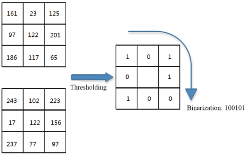
As shown in Figure 2, the same LBP code value was obtained through differential comparison and binarization for two local neighborhoods, which lie at different positions and differ sharply in texture feature. This indicates that the LBP operator loses part of the texture information during the extraction of texture features.
Figure 2. The loss of texture information
Therefore, the encoding method of the basic LBP operator was improved by comparing the mean grayscales and mean differential amplitudes of the local neighborhood and the global image.
3.2 Improved LBP operator
3.2.1 Encoding strategy
The encoding strategy is a three-stage process: the possible texture directions in the local neighborhood are grouped, the spatial template of each possible direction is used to differentiate the central pixel from each local pixel, and the direction and amplitude of the difference are included in the encoding process.
In the local neighborhood, there are three possible texture directions: edge texture, rectangular texture and oblique angle texture. For each texture, four spatial templates are needed to calculate the corresponding LBP code value.
For edge texture encoding, the LBP code value can be calculated by:
$\begin{aligned}
L B P_{L 1}^{C D}=\sum_{i=0}^{C / 2-1}(&\left.u\left(g_{i}-g_{0}\right) \odot u\left(g_{o}-g_{i+C / 2}\right)\right) 2^{2 i} \\
&+u\left(\left(g_{i}-g_{o}\right)\right.\\
&\left.\left.-\left(g_{o}-g_{i+c / 2}\right)\right) 2^{2 i+1}\right)
\end{aligned}$ (4)
where, $u\left(g_{i}-g_{o}\right) \odot u\left(g_{o}-g_{i+c / 2}\right)$ is the possible directions of edge texture, i.e. 0°, 45°, 90°, and 135°; $u\left(\left(g_{i}-g_{o}\right)-\left(g_{o}-g_{i+c / 2}\right)\right)$ is the trend of grayscale intensity in the current texture direction.
For rectangular texture encoding, the LBP code value can be calculated by:
$\begin{aligned}
L B P_{L 2}^{C D}=\sum_{i=0}^{C / 2-1} &\left(\left(u\left(g_{2 i-1}-g_{o}\right) \odot u\left(g_{o}-g_{2 i+1}\right)\right) 2^{2 i}\right.\\
&+u\left(\left(g_{2 i-1}-g_{o}\right)\right.\\
&\left.\left.-\left(g_{o}-g_{2 i+1}\right)\right) 2^{2 i+1}\right)
\end{aligned}$ (5)
where, $u\left(g_{2 i-1}-g_{o}\right) \odot u\left(g_{o}-g_{2 i+1}\right)$ is the possible directions of rectangular texture; $u\left(\left(g_{2 i-1}-g_{o}\right)-\left(g_{o}-g_{2 i+1}\right)\right)$ is the trend of grayscale intensity in the current texture direction.
For oblique angle texture encoding, the LBP code value can be calculated by:
$\begin{array}{c}
L B P_{L 3}^{C D}=\sum_{i=0}^{C / 2-1}\left(\left(u\left(g_{2 i}-g_{o}\right) \odot u\left(g_{0}-g_{2 i+2}\right)\right) 2^{2 i}\right. \\
+u\left(\left(g_{2 i}-g_{o}\right)\right. \\
\left.\left.-\left(g_{o}-g_{2 i+2}\right)\right) 2^{2 i+1}\right)
\end{array}$ (6)
where, $u\left(g_{2 i}-g_{o}\right) \odot u\left(g_{o}-g_{2 i+2}\right)$ is the possible directions of oblique angle texture; $u\left(\left(g_{2 i}-g_{o}\right)-\left(g_{o}-g_{2 i+2}\right)\right)$ is the trend of grayscale intensity in the current texture direction.
The traditional LBP operator only emphasizes on the texture information in the local neighborhood, failing to consider the correlation and difference between local and global grayscales. Here, the comparison between local and global grayscales is added to improve the recognition performance of the LBP operator.
First, the comparison between local and global grayscales can be encoded by:
$L B P_{a v g}^{C D}=u\left(\sum_{i=0}^{C-1}\left(g_{i}+g_{o}\right) / C+1-\sum_{i=0}^{N-1} g_{i} / N\right)$ (7)
where, $\sum_{i=0}^{C-1}\left(g_{i}+g_{o}\right) / C+1$ is the mean grayscale of the (C+1) pixels in the local neighborhood of the current central pixel; $\sum_{i=0}^{N-1} g_{i} / N$ is the global mean grayscale of the image.
Next, the comparison between the mean change amplitudes of local and global grayscales can be encoded by:
$\begin{aligned}
L B P_{\operatorname{mag}}^{C D}=u\left(\sum_{i=0}^{C-1}\right.& a b x\left(g_{i}-g_{o}\right) / C \\
&\left.-\sum_{i=0}^{N-1} \sum_{i=0}^{C-1} a b s\left(g_{i}-g_{o}\right) / N \times C\right)
\end{aligned}$ (8)
where, $\sum_{i=0}^{C-1} a b x\left(g_{i}-g_{o}\right) / C$ is the mean change amplitude of the C neighborhood pixels and the central pixel in the local neighborhood after grayscale difference; $\left.\sum_{i=0}^{N-1} \sum_{i=0}^{C-1} a b s\left(g_{i}-g_{o}\right) / N \times C\right)$ is the global mean amplitude of the whole image after the grayscale difference of C-neighborhood.
Then, an improved LBP operator encoding was formed by concatenating three groups of sub-codes of local texture encodings ($L B P_{L 1}^{C D}, L B P_{L 2}^{C D}, L B P_{L 3}^{C D}$) and two groups of sub-codes of global comparison information encodings $\left(L B P_{a v g}^{C D}, L B P_{\operatorname{mag}}^{C D}\right)$. The improved LBP operator not only reflects the local features like texture direction and grayscale trend, but also contains the global features of the entire image. It can extract richer texture information, and achieve better discriminability.
The standard LBPC,R operator can generate 2C patterns (code values). For example, 256 patterns will be generated if C=8. Obviously, it is not suitable to directly take the output of the standard operator as the final eigenvector. Meanwhile, $L B P_{C, R}^{t^{i}}$ can reduce the total number of patterns to 36, and $L B P_{C, R}^{U}$ can lower that number to 59.
The above operators modify the encoding pattern of the LBP operator to varied degrees. Choosing an operator means accepting the corresponding modified encoding pattern. To select the most discriminable pattern class, the following factors were fully considered: the similarity and difference between images, the occurrence probabilities of different patterns, the consistency of pattern distribution, and the contribution of class information to pattern selection.
After the features of a texture image have been extracted by the LBP operator, the probability for each pattern to appear in the image was counted. The patterns with high probabilities were treated as the main patterns that illustrate image texture, while those with low probabilities were deemed as irrelevant information or noise. Next, the consistency of pattern distribution was measured, that is, the variation in the number of the same pattern appearing in different images. If the pattern distribution is relatively consistent, the pattern was regarded as the image background. On this basis, the authors designed a pattern selection strategy based on the weighted ranking of classes:
First, the original LBP patterns of the training set are grouped into different classes. Then, the occurrence probability and standard deviation of each pattern are calculated for each class. According to the standard deviation, different weights are assigned to the occurrence probabilities of different patterns. After that, the weighted occurrence probabilities are ranked in descending order. Finally, the main patterns of different classes of images are combined as the final main pattern eigenvector. The above process can be mathematically described as follows:
Step 1. Initialize a set of N training images S={X1, X2, …, XN}, and the LBP pattern vector of each image Xi=(v1, v2, …, vM), where vi is the times that the LBP pattern appears in the current image.
Step 2. Set the number C of the possible classes of the current image, and categorize the image set S into C classes, such that the same images fall into the same class $S_{C_{i}}=\left\{X_{1}, X_{2}, \ldots, X_{N_{i}}\right\}$, Ci=1, 2, …, C.
Step 3. Calculate the total number of occurrences of each LBP pattern: $\text { TotalHist }_{c_{i}, i}=\sum_{X_{i=1}}^{N 1} v_{i, X_{i}} X_{i}$ , and the standard deviation of each LBP pattern: $\text { SDHist }_{c_{i}, i}=\text { StandardDeviation}\left(v_{i, X_{1}}, v_{i, X_{2}}, \ldots, v_{i, X_{N}}\right)$ .
Step 4. Assign a weight to the occurrence probability of each pattern based on the standard deviation.
Step 5. Calculate the weighted probability of each, sort the new image set $\vec{S}$ in descending order of the weighted probability, and take the top k patterns as the main patterns of the current class.
Step 7. Select the k main patterns of each class $S_{C_{i}}$ in turn by Steps 3-5, and record the $\vec{k}_{C_{1}}$ value of the selected patterns.
Step 8. For the eigenvector set S of LBP patterns of the original image, take the pattern class corresponding to ktotal as the final eigenvector of main patterns.
Classification is an important step of image recognition. The recognition performance hinges on the classifier performance. In this paper, the SVM classifier is selected to recognize the image of bolt loss in underground pipelines, and the swarm intelligence algorithm [20] is introduced to optimize the SVM parameters.
4.1 Parameter optimization
The classification performance of the SVM mainly depends on kernel selection and parameter setting. If the kernel function or parameters is improper, the SVM will experience performance degradation, and even lose the ability to classify samples. Despite being a hot topic, there is not yet a widely recognized theory on the selection of the kernel function and parameters of the SVM. In practical application, the kernel function is basically determined by experience.
In most cases, radial basis function (RBF) is the most superior kernel function for the SVM. But the two SVM parameters, namely, the penalty function and the kernel width, are difficult to determine. The ideal values of the two parameters can only be ascertained by traversing the entire search space. To optimize the SVM parameters, this paper improves the optimization strategy and adaptive phase of a swarm intelligence search algorithm called teaching-learning-based optimization (TLBO) algorithm [21]. The improvement aims to speed up the convergence, maintain the population diversity in the search process, and enhance the ability to jump out of the local optimum trap.
The TLBO algorithm is mainly improved in three aspects: (1) the judgement of whether to update the knowledge of the current student after each round of learning was improved from individual greedy strategy to class optimal strategy; (2) a self-adaptive learning phase was designed, in which the adaptive learning step size and knowledge level can be adjusted as per the current knowledge level of students; (3) a self-adaptive communication phase was designed to change the learning between two students into that between three students.
In the standard TLBO algorithm, each student is reset into a freshman after the current round of learning, and immediately compared with each student who has not learned anything (hereinafter referred to as unlearned student). According to the greedy strategy, the student with the better performance is retained in the next round. Focusing on individual renewal, the greedy strategy might eliminate some high-quality individuals, while retaining a few inferior individuals. Thus, the convergence of the entire population might be slowed down. To solve the problem, this paper optimizes the greedy strategy into class optimal strategy, drawing on the principle of group updating. First, all freshmen and unlearned students form a class at the end of the current round of learning, and all the students in the class are ranked by score. Then, only the students with relatively high scores in the class are retained for the new class in the next round.
In the teaching stage, the students mainly accept the knowledge imparted by the teacher. During actual learning, however, the students often differ in performance and the knowledge gap with the teacher. Each student ought to learn from the teacher based on his/her knowledge level. In the standard TLBO algorithm, the learning step size of each student is randomly assigned, rather than adjusted as per the individual situation. This paper designs an adaptive learning step size, allowing each student to adjust the size as per his/her knowledge gap with the teacher. The adjustment process can be described mathematically as:
In the i-th iteration, the adaptive learning step size w was added when student a is learning the knowledge of subject k:
$w=R_{\text {best}}-R_{a} / R_{\text {best}}-R_{\text {worst}}$ (9)
where, Ra is the score of student a; Rbest is the best score in the current class; Rworst is the worst score in the current class.
The improved knowledge update method for student a can be expressed as:
$\text { Diff_Mean }_{k, a, i}^{\text {new}}=w \times\left(T_{k, i}-T_{F} M_{k, i}\right)$ (10)
where, Mk,i is the mean knowledge level of the current class.
In this way, student a can adjust his/her learning step size as per his/her knowledge gap with the teacher.
In the teaching stage, the teacher attempts to increase the mean knowledge level Mk,i of the current class Mk,i. But the students tend to vary in the knowledge gap with the teacher. The variation cannot be reflected by the mean knowledge level Mk,i. This paper proposes an adaptive knowledge level, enabling each student to adjust the learning progress as per his/her knowledge gap with the teacher. The adjustment process can be described mathematically as:
In the i-th iteration, the adaptive knowledge level $M_{k, i}^{n e w}$ was added when student a is learning the knowledge of subject k:
$M_{k, i}^{\text {new}}=T_{k, i}+a_{k, i} / 2$ (11)
where, ak,i is the knowledge level of student a on subject k; Tk,i is the knowledge level of the teacher on subject k.
In this way, student a can adjust his/her knowledge level as per his/her knowledge gap with the teacher.
In the standard TLBO algorithm, student a randomly selects a student b as the object in the student communication stage. If student b does better, student a will move towards him/her; If student b does poorer, student a will move away from him/her. To broaden student knowledge and improve population diversity, the number of students engaged in the communication was increased from 2 to 3.
In the i-th iteration, the current student a learns from students b and c, both of who are doing better than student a on subject k, to adjust his/her learning step size through autonomous learning:
$L_{k, a, i}^{n e w}=L_{k, a, i}+(2 \times r-1)\left|L_{k, b, i}-L_{k, c, i}\right|$ (12)
where, r is a random number within [0, 1].
If student a falls between b and c in terms of score, he/she will adjust his/her learning strategy towards that of the other two student. In the i-th iteration, suppose student b has the highest score, a has the middle score, and c has the lowest score. In this case, the current student a will learn from the experience of b and the lesson of c, and exchange knowledge with them on subject k. This process can be mathematically described as:
$\begin{array}{c}
L_{k, a, i}^{n e w} \\
=L_{k, a, i}+r_{b}\left(L_{k, b, i}-L_{k, a, i}\right)-r_{c}\left(L_{k, c, i}-L_{k, a, i}\right)
\end{array}$ (13)
where, rb and rc are random numbers within [0, 1].
4.2 Image recognition based on Gabor transform
Gabor wavelet [22] has a perceptual response similar to human visual system, and a good resolution in both spatial and frequency domains. This paper selects the kernel function of Gabor wavelet to convolute the original image. In this way, an image matrix with 40 complex coefficients was extracted, reflecting the features of the original images in different frequency scales and texture directions.
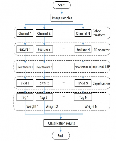
Gabor wavelet transform can achieve the best localization effect in both time domain and frequency domain. However, the dimension of the eigenvectors obtained by Gabor wavelet transform is 40 times of the original image, a taletelling sign of high redundancy. This seriously suppresses the recognition efficiency. Meanwhile, the texture features extracted by LBP operator are robust to angle and occlusion changes, and strongly discriminable. Therefore, Gabor transform was applied to the original image to obtain the response image in 5 scales and 8 directions. Then, the improved LBP operator was implemented to extract the eigenvectors of different channels. After that, the 40 groups of eigenvectors were optimized to obtain better recognition performance. Figure 3 explains the processes of the improved classification algorithm for bolt loss recognition.
Figure 3. The overall processes of improved classification algorithm for bolt loss recognition
After Gabor transform of the original image, a total of 40 response images could be obtained in different channels. Then, the LBP operator was applied for feature extraction, producing a 112-dimensional eigenvector in each channel. Obviously, the 40×112 dimensional eigenvector cannot be directly recognized by the SVM classifier. Therefore, the improved LBP operator was called to select the main patterns of the 40 channel eigenvectors. The optimal feature combination of each channel was obtained through separate recognition of each channel. Table 1 records the optimal feature retention dimension and recognition rate of each channel.
Table 1. The optimal feature retention dimension and recognition rate of each channel
|
Channel |
Dimension |
Recognition rate (%) |
|
1 |
38 |
58.76 |
|
2 |
40 |
54.11 |
|
3 |
39 |
54.11 |
|
4 |
41 |
51.25 |
|
5 |
37 |
62.31 |
|
6 |
42 |
57.26 |
|
7 |
41 |
52.73 |
|
8 |
42 |
58.32 |
|
9 |
28 |
60.51 |
|
10 |
37 |
60.38 |
|
11 |
36 |
64.57 |
|
12 |
38 |
63.35 |
|
13 |
31 |
71.75 |
|
14 |
38 |
60.12 |
|
15 |
37 |
62.87 |
|
16 |
38 |
57.92 |
|
17 |
22 |
60.30 |
|
18 |
31 |
71.58 |
|
19 |
33 |
60.83 |
|
20 |
27 |
55.82 |
|
21 |
25 |
63.82 |
|
22 |
40 |
68.90 |
|
23 |
31 |
72.51 |
|
24 |
32 |
87.34 |
|
25 |
17 |
82.62 |
|
26 |
32 |
71.93 |
|
27 |
28 |
76.82 |
|
28 |
30 |
78.37 |
|
29 |
17 |
78.17 |
|
30 |
31 |
65.83 |
|
31 |
27 |
55.90 |
|
32 |
33 |
80.49 |
|
33 |
11 |
89.20 |
|
34 |
20 |
89.10 |
|
35 |
19 |
82.93 |
|
36 |
10 |
88.59 |
|
37 |
17 |
81.72 |
|
38 |
18 |
85.73 |
|
39 |
21 |
84.85 |
|
40 |
19 |
90.77 |
As shown in Table 1, the recognition rates of different channels differed sharply. The performance of our algorithm can be greatly improved by optimizing the combination of eigenvectors.
After optimal combination of eigenvectors was determined for each channel, the SVM classifier was adopted to identify the eigenvectors of each channel, and different weights were assigned to the predicted class tags of each channel. To test the effects of the weighting process on the recognition performance, the recognition rates of our algorithm were compared with different weight optimization methods: no weight optimization, taking recognition rate as weight, adaptive boost, and the improved TLBO. The experimental results are shown in Table 2.
Table 2. The recognition rates with different weight optimization methods
|
Weight optimization method |
Recognition rate (%) |
|
No weight optimization |
97.52 |
|
Taking recognition rate as weight |
97.55 |
|
Adaptive boost |
98.16 |
|
Improved TLBO |
99.03 |
As shown in Table 2, the improved TLBO led to better results than the other two weight optimization methods, in terms of search ability and recognition accuracy. The weight optimization by the improved TLBO provides a good basis for pattern classification and image recognition.
To realize automatic detection of bolt loss images of underground pipelines, this paper establishes a recognition algorithm that can effectiveness identify the images of key parts of underground pipelines. The main innovation is the design of an improved LBP operator for the extraction of texture features. To enhance the texture discriminability, the local texture features were compared with global features, and the comparative results were included in the encoding method. In addition, the TLBO algorithm was improved to optimize multiple parameters of the SVM, which improves the convergence speed and optimization accuracy of the recognition algorithm.
[1] Richmond, N.J., Willett, P., Clark, R.D. (2004). Alignment of three-dimensional molecules using an image recognition algorithm. Journal of Molecular Graphics and Modelling, 23(2): 199-209. https://doi.org/10.1016/j.jmgm.2004.04.004
[2] Chen, J., Zhan, Y., Cao, H., Wu, X. (2018). Adaptive probability filter for removing salt and pepper noises. IET Image Processing, 12(6): 863-871. https://doi.org/10.1049/iet-ipr.2017.0910
[3] Du, H. (2018). Research on image de-disturbing algorithm based on dark channel prior and anisotropic Gaussian filtering. Concurrency and Computation: Practice and Experience, 30(24): e4933.1-e4933.11. https://doi.org/10.1002/cpe.4933
[4] Schmeing, M., Jiang, X. (2014). Edge-aware depth image filtering using color segmentation. Pattern Recognition Letters, 50: 63-71. https://doi.org/10.1016/j.patrec.2014.03.026
[5] Zhu, H., Morris, J.S., Wei, F., Cox, D.D. (2017). Multivariate functional response regression, with application to fluorescence spectroscopy in a cervical pre-cancer study. Computational Statistics & Data Analysis, 111: 88-101. https://doi.org/10.1016/j.csda.2017.02.004
[6] Zhao, Y., Jia, W., Hu, R. X., Min, H. (2013). Completed robust local binary pattern for texture classification. Neurocomputing, 106: 68-76. https://doi.org/10.1016/j.neucom.2012.10.017
[7] Prakash, K.N., Prasad, K.S. (2013). Sign LTP and magnitude LTP for image indexing and retrieval. International Journal of Signal and Imaging Systems Engineering, 6(4): 227-239. https://doi.org/10.1504/IJSISE.2013.056635
[8] Guo, Z., Zhang, L., Zhang, D. (2010). A completed modeling of local binary pattern operator for texture classification. IEEE Transactions on Image Processing, 19(6): 1657-1663. https://doi.org/10.1109/TIP.2010.2044957
[9] Yang, S.H., Chen, Y.P. (2012). An evolutionary constructive and pruning algorithm for artificial neural networks and its prediction applications. Neurocomputing, 86: 140-149. https://doi.org/10.1016/j.neucom.2012.01.024
[10] Yuan, Q., Zhou, W., Xu, F., Leng, Y., Wei, D. (2018). Epileptic EEG identification via LBP operators on wavelet coefficients. International Journal of Neural Systems, 28(8): 1850010. https://doi.org/10.1142/S0129065718500107
[11] Zhu, C., Bichot, C.E., Chen, L. (2013). Image region description using orthogonal combination of local binary patterns enhanced with color information. Pattern Recognition, 46(7): 1949-1963. https://doi.org/10.1016/j.patcog.2013.01.003
[12] Datta Rakshit, R., Nath, S.C., Kisku, D.R. (2017). An improved local pattern descriptor for biometrics face encoding: a LC–LBP approach toward face identification. Journal of the Chinese Institute of Engineers, 40(1): 82-92. https://doi.org/10.1080/02533839.2016.1259020
[13] Chinnam, S.K.R., Sistla, V., Kolli, V.K.K. (2019). SVM-PUK kernel based MRI-brain tumor identification using texture and Gabor wavelets. Traitement du Signal, 36(2): 185-191. https://doi.org/10.18280/ts.360209
[14] Thanh Noi, P., Kappas, M. (2018). Comparison of random forest, k-nearest neighbor, and support vector machine classifiers for land cover classification using Sentinel-2 imagery. Sensors, 18(1): 18. https://doi.org/10.3390/s18010018
[15] Richhariya, B., Tanveer, M. (2018). EEG signal classification using universum support vector machine. Expert Systems with Applications, 106: 169-182. https://doi.org/10.1016/j.eswa.2018.03.053
[16] Mo, H., Zhao, Y. (2016). Motor imagery electroencephalograph classification based on optimized support vector machine by magnetic bacteria optimization algorithm. Neural Processing Letters, 44(1): 185-197. https://doi.org/10.1007/s11063-015-9469-7
[17] Wang, X., Luo, F., Sang, C., Zeng, J., Hirokawa, S. (2017). Personalized movie recommendation system based on support vector machine and improved particle swarm optimization. IEICE Transactions on Information and Systems, 100(2): 285-293. https://doi.org/10.1587/transinf.2016EDP7054
[18] Montiel, L.A.H. (2016). Hybrid algorithm applied on gene selection and classification from different diseases. IEEE Latin America Transactions, 14(2): 930-935.
[19] Ojala, T., Pietikäinen, M., Harwood, D. (1996). A comparative study of texture measures with classification based on featured distributions. Pattern recognition, 29(1): 51-59. https://doi.org/10.1016/0031-3203(95)00067-4
[20] Zhou, H., Wang, R., Wang, C. (2008). A novel extended local-binary-pattern operator for texture analysis. Information Sciences, 178(22): 4314-4325. https://doi.org/10.1016/j.ins.2008.07.015
[21] Baykasoğlu, A., Hamzadayi, A., Köse, S.Y. (2014). Testing the performance of teaching–learning based optimization (TLBO) algorithm on combinatorial problems: Flow shop and job shop scheduling cases. Information Sciences, 276: 204-218. https://doi.org/10.1016/j.ins.2014.02.056
[22] Liu, Y., Yang, H., Sun, G.X., Bin, S. (2020). Collaborative filtering recommendation algorithm based on multi-relationship social network. Ingénierie des Systèmes d’Information, 25(3): 359-364. https://doi.org/10.18280/isi.250310