Shizhen Bai | Fuli Han*
© 2020 IIETA. This article is published by IIETA and is licensed under the CC BY 4.0 license (http://creativecommons.org/licenses/by/4.0/).
OPEN ACCESS
The monitoring of tourist behaviors, coupled with the recognition of scenic spots, greatly improves the quality and safety of travel. The visual information is the underlying features of scenic spot images, but the semantics of the information have not been satisfactorily classified or described. Based on image processing technologies, this paper presents a novel method for scenic spot retrieval and tourist behavior recognition. Firstly, the framework of scenic spot image retrieval was constructed, followed by a detailed introduction to the extraction of scale invariant feature transform (SIFT) features. The SIFT feature extraction includes five steps: scale space construction, local space extreme point detection, precise positioning of key points, determination of key point size and direction, and generation of SIFT descriptor. Next, multiple correlated images were mined for the target scenic spot image, and the feature matching method between the target image and the set of scenic spot images was introduced in details. On this basis, a tourist behavior recognition method was designed based on temporal and spatial consistency. The proposed method was proved effective through experiments. The research results provide theoretical reference for image retrieval and behavior recognition in many other fields.
image processing, scenic spot image retrieval, tourist behavior recognition, scale invariant feature transform (SIFT)
The development of Internet technology has diversified the tourist demand for information services of scenic spots. More and more tourists are acquiring scenic spot information from the Internet, and actively sharing their travel photos with others [1-4]. Many travel photos contain the visual features of scenic spots, which reflect the background knowledge of the scenic spots and provide a wealth of relevant information (e.g. nearby stores, environment, and traffic conditions). Therefore, many domestic and foreign scholars have explored scenic spot recognition and retrieval based on image processing [5-8].
With the proliferation of video surveillance system, tourist behaviors can now be monitored intelligently by advanced computer image processing technologies. The monitoring of tourist behaviors, coupled with the recognition of scenic spots, promotes the digital management of tourist spots, improves the quality and safety of travel, and contributes greatly to the sustainable development of tourist spots [9, 10].
So far, many scholars have mined and analyzed the images on scenic spots and tourist behaviors, laying the basis for scenic spot retrieval, landmark recognition and labeling, scenic spot image classification, as well as the optimization and recommendation of travel routes [10, 11]. Srivastava et al. [12] optimized the content-based image classification method for scenic spot images, and greatly improved the classification accuracy of scenic spot images. Kasban and Salama [13] constructed a client/server (C/S) architecture of scenic spot image, and classified scenic spots into different categories based on their images. Following probabilistic latent semantic analysis (PLSA) and hypergraph method, Muhammad and Baik [14] carried out semantic analysis of scenic spot images, explored the relationships between global positioning system (GPS) information, labels, and visual semantics of scenic spots, and verified the accuracy of image-based scenic spot recommendation through a recognition experiment on 50,000+ scenic spot images from social networks. Erkut et al. [15] built the architecture of an image-based real-time search system for diverse information of scenic spots, and generated a personalized introduction summary containing scenic spot images from various angles for numerous scenic spots, providing users with an excellent search experience. Based on tourism big data, Hu et al. [16] established an image location recognition system on the Hadoop distributed platform, optimized the search keywords and image indexing method, and successfully located scenic spots with a massive number of scenic spot images.
Currently, tourist behavior patterns are mainly studied based on the spatiotemporal information and behavior features of tourists [17, 18]. From social networks, Fan et al. [19] collected more than 3,000 travel photos uploaded by tourists to Hainan, analyzed the tourist behavior patterns in view of the images, the relevant GPS coordinates, and shooting time, and disclosed the correlations between tourist flow, hot scenic spots, and uncivilized behaviors. Mabrouk and Zagrouba [20] integrated geographical and time information into the analysis of the spatiotemporal behavior patterns of tourists in the Forbidden City, examined the factors affecting the travel routes, and summed up four core influencing factors: time, space, scenic spot, and path trajectory.
Some researchers have introduced image processing technologies to recognize the tourist behaviors in surveillance videos through experiments [21-23]. Mabrouk and Zagrouba [20] maximized the naive Bayesian mutual information based on the spatiotemporal points of interest, in an attempt to enhance the recognition accuracy of tourist behaviors in surveillance images on scenic spots. Ahmad et al. [24] recognized 25 kinds of continuous actions of human body, and applied the recognition method to identify the tourist behaviors in scenic spots.
In scenic spot images, the visual information is the underlying features. The semantics of the information have not been satisfactorily classified or described. Relying on image processing technologies, this paper improves the effectiveness of scenic spot retrieval and tourist behavior recognition. Firstly, the framework of scenic spot image retrieval was constructed, followed by the explanation of the extraction of scale invariant feature transform (SIFT) features. Next, multiple correlated images were mined for the target scenic spot image, and the feature matching method between the target image and the set of scenic spot images was introduced in details. On this basis, a tourist behavior recognition method was designed based on temporal and spatial consistency, plus its implementation process. The proposed method was proved effective through experiments.
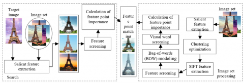
Figure 1 presents the framework of our scenic spot image retrieval method. The extraction of global and local features, the weighting of multiple correlated images, and the feature matching with the set of scenic spot images will be detailed in turn.
Figure 1. The framework of scenic spot image retrieval
2.1 SIFT feature extraction
SIFT is a popular local feature detection method in image retrieval, thanks to its robustness, versatility, scalability, fast speed, and strong discriminability. SIFT feature extraction can be broken down into five steps, namely, scale space construction, local space extreme point detection, precise positioning of key points, determination of key point size and direction, and generation of SIFT descriptor. In the context of scenic spot images, the five steps of SIFT feature extraction are described as follows:
(1) Scale space construction
To extract features from scenic spot images at different resolutions, the scale space representation sequence of the target scenic spot image can be constructed through multi-scale transform under different scales. The scale space expression A(a,b,ε) of a two-dimensional (2D) image A(a,b) can be obtained through the transform with a 2D Gaussian kernel G(a,b,ε):
$\begin{align} & A(a,b,\varepsilon )=G(a,b,\varepsilon )*A\left( a,b \right) \\ & =\frac{1}{2\pi {{\varepsilon }^{2}}}{{e}^{-\left( {{a}^{2}}+{{b}^{2}} \right)/2{{\varepsilon }^{2}}}}*A\left( a,b \right) \\ \end{align}$ (1)
where, * is the sign of convolution; (a,b) is the coordinates of a pixel in the scenic spot image; ε is the scale space factor. The ε value directly affects the blur degree of the transformed image. Compared with the Laplacian of Gaussian (LoG) operator, the Gaussian difference scale space, which approximates the scale-normalized LoG function, can detect key points effectively and stably. The Gaussian difference scale space can be calculated by:
$\begin{align} & S\left( x,y,\sigma \right)=\left[ G(a,b,n\varepsilon )-G(a,b,\varepsilon ) \right]*A\left( a,b \right) \\ & =A(a,b,n\varepsilon )-A(a,b,\varepsilon ) \\ \end{align}$ (2)
(2) Local space extreme point detection
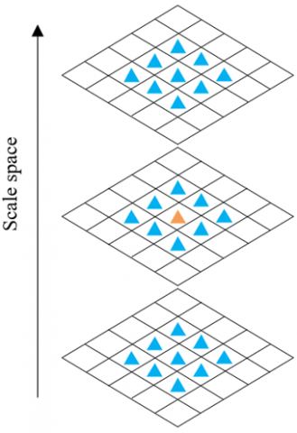
The location of the extreme point in the local space is to search for the minimum and maximum within the given range. During the search, each pixel should be compared with the adjacent pixels, to see whether it is an extreme point in its neighborhood. The local space extreme point detection process is illustrated in Figure 2, in which the orange pixel in the middle layer needs to be compared with 8 pixels in the same scale, and the 9 pixels in the adjacent scales on the upper and lower layers.
Figure 2. The sketch map of local space extreme point detection
(3) Precise positioning of key points
Among the extreme points, the unstable points on the edges and those with grayscale mutations must be removed. Each key point can be located precisely by fitting the LoG operator with the three-dimensional (3D) quadratic formula:
$P\left( e \right)=P+\frac{\partial {{P}^{\lambda }}}{\partial E}E+\frac{1}{2}{{E}^{\lambda }}\frac{{{\partial }^{2}}P}{\partial {{E}^{2}}}E$ (3)
By deriving the above formula and making the result zero, the desired extreme point can be obtained:
$e=-\frac{{{\partial }^{2}}{{P}^{-1}}}{\partial {{E}^{2}}}\cdot \frac{\partial P}{\partial E}$ (4)
The position of the corresponding extreme point can be expressed as:
$P\left( e \right)=P+\frac{1\partial {{P}^{\lambda }}}{2\partial E}E$ (5)
If P(x) is smaller than the set threshold, the extreme point will be removed; if it is greater than the threshold, the extreme point must have a high contrast and will be retained.
For an edge point, if its main curvature is small on the vertical edge and large on the horizontal edge, then it must be poor in decision-making and are susceptible to noise. The main curvature can be solved by the second-order Hessian matrix:
$H=\left[ \begin{matrix} {{h}_{xx}} & {{h}_{xy}} \\ {{h}_{xy}} & {{h}_{yy}} \\\end{matrix} \right]$ (6)
Let δ and τ be the eigenvalues of the Hessian matrix corresponding to the gradients in the x and y directions, respectively. Then, the following equation can be derived:
$\frac{Tr{{\left( H \right)}^{2}}}{Det\left( H \right)}=\frac{{{\left( {{h}_{xx}}+{{h}_{yy}} \right)}^{2}}}{{{h}_{xx}}{{h}_{yy}}-{{\left( {{h}_{xy}} \right)}^{2}}}=\frac{{{\left( \delta +\tau \right)}^{2}}}{\delta \tau }$ (7)
If δ and τ correspond to relatively large and small eigenvalues, respectively. Let ρ be the ratio of δ to τ. Then, formula (7) can be rewritten as:
$\frac{Tr{{\left( H \right)}^{2}}}{Det\left( H \right)}=\frac{{{\left( \rho \tau +\tau \right)}^{2}}}{\rho {{\tau }^{2}}}=\frac{{{\left( \rho +1 \right)}^{2}}}{\rho }$ (8)
As shown in formula (8), (ρ+1)2/ρ increases with ρ, and minimizes at ρ=1. Since ρ is positively correlated with the gradients in the x and y directions, the point must be an edge point that should be removed, as long as the threshold of ρ satisfies the inequality below:
$\frac{Tr{{\left( H \right)}^{2}}}{Det\left( H \right)}\ge \frac{{{\left( \rho +1 \right)}^{2}}}{\rho }$ (9)
(4) Determination of key point size and direction
To make the feature descriptor invariant to rotation, each key point needs to be assigned a direction. The modulus and gradient direction of each key point can be respectively expressed as:
$M\left( a,b \right)=\sqrt{\begin{align} & {{\left( A\left( a+1,b \right)-A\left( a-1,b \right) \right)}^{2}} \\ & +{{\left( A\left( a,b+1 \right)-A\left( a,b-1 \right) \right)}^{2}} \\ \end{align}}$ (10)
$\alpha \left( a,b \right)={{\tan }^{-1}}\left( \frac{A\left( a,b+1 \right)-A\left( a,b-1 \right)}{A\left( a+1,b \right)-A\left( a-1,b \right)} \right)$ (11)
(5) Generation of SIFT descriptor
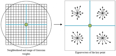
Based on the direction of a key point, a coordinate axis should be set up to measure the direction of its neighboring pixels, and a 16×16 area should be established with the key point as the center. The generation of SIFT descriptor is explained in Figure 3, where the central point is the key point, the circle is the range of Gaussian weights, and the adjacent squares of the key point are the adjacent pixels on the same scale.
As shown in Figure 3, the 128-dimansional descriptor of the key point encompasses 16 sub-key points and the corresponding 8 directions. In each square, the length of the arrow, which indicates the gradient direction, represents the gradient modulus of the corresponding pixel. With the aid of the histogram, the gradients in each 8×8 area can be counted, and the cumulative results can be obtained for each sub-key point.
Figure 3. The sketch map of SIFT descriptor generation
2.2 Weight calculation for multiple correlated images and feature matching with image set
Before mining the multiple correlated images for the target scenic spot image, it is necessary to extract the wavelet packet descriptor and color moment of that image. Here, the 2D wavelet transform method of Harr transform is implemented to generate a 180-dimensional eigenvector. The corresponding wavelet packet descriptor can be obtained by:
$\gamma _{i}^{k}=\frac{1}{h\times w}\sum\limits_{a=1}^{h}{\sum\limits_{b=1}^{w}{\left| \omega _{i}^{k}\left( a,b \right) \right|}}\text{ }$ (12)
$\beta _{i}^{k}=\sqrt{\frac{1}{h\times w}\sum\limits_{a=1}^{h}{\sum\limits_{b=1}^{w}{{{\left( \omega _{i}^{k}\left( a,b \right)-\gamma _{i}^{k} \right)}^{2}}}}}$ (13)
$W\left( K \right)=\left( \gamma _{1}^{K},\beta _{1}^{K},\cdots ,\gamma _{64}^{K},\beta _{64}^{K} \right) $ (14)
${{W}^{*}}\left( K \right)=\left[ W\left( 0 \right),\cdots ,W\left( K \right) \right]$ (15)
where, ik(a,b) is the coefficient of coefficient of the pixel (a,b) on the i-th sub-image after the Harr transform; h and w are the height and width of the sub-image, respectively. Let M be the total number of pixels; plj be the appearance probability of the pixel with grayscale l in the component of the j-th color channel. Then, the color moment of the target image can be defined by:
${{\eta }_{j}}=\frac{1}{M}\sum\limits_{l=1}^{M}{p_{j}^{l}}\text{ }$ (16)
${{\mu }_{j}}=\sqrt{\frac{1}{M}\sum\limits_{l=1}^{M}{{{\left( p_{j}^{l}-{{\eta }_{i}} \right)}^{2}}}}$ (17)
${{\zeta }_{j}}=\sqrt[3]{\frac{1}{M}\sum\limits_{l=1}^{M}{{{\left( p_{j}^{l}-{{\eta }_{i}} \right)}^{3}}}}$ (18)
The RGB (red, green, blue) color moment of the image can be described by the 9-dimensional color features below:
$C=\left[ \eta R,\mu R,\zeta R,\eta G,\mu G,\zeta G,\eta B,\mu B,\zeta B \right]$ (19)
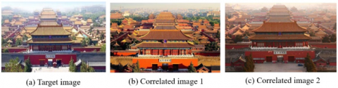
The next step is to calculate the Euclidean distance between the global descriptor of the target image and that of each image in the image set (hereinafter referred to as the contrastive image). If the distance is smaller than the set threshold, the contrastive image is one of the multiple correlated images of the target image. Figure 4 provides an example of the target image and its correlated images.
Figure 4. The mining of multiple correlated images
After the correlated images are selected, the SIFT features were extracted from each image by the process mentioned in subsection 2.1. Then, all SIFT features were classified by k-means clustering (KMC). Let SIFTd be the d-th SIFT feature point of the target image. Then, each feature of the target image possesses the following information:
$SIF{{T}_{d}}=\left\{ s_{1}^{1},\ldots ,s_{1}^{{{\theta }_{1}}},\ldots ,s_{i}^{1},\ldots ,s_{i}^{{{\theta }_{i}}},\ldots ,s_{m}^{1},\ldots ,s_{m}^{{{\theta }_{m}}} \right\}$ (20)
where, sθii is the θi-th SIFT feature point of the i-th correlated image in the class of SIFTd. Once the feature points of the target image have been screened, those of contrastive images should also be screened. In this paper, quantitative dimensionality reduction is combined with mage content clustering to select the useful visual words from the image set. To speed up the retrieval process and optimize the retrieval performance, three steps were designed to screen the useful visual words:
Step 1: Each image is compressed vertically and horizontally. Then, the feature points are extracted again from the compressed image. The similarity between the descriptors of the original and compressed images can be calculated by:
$sim\left( {{A}_{b}},{{A}_{a}} \right)={{A}_{b}}*{{A}_{a}}/\left( \left\| {{A}_{b}} \right\|\times \left\| {{A}_{a}} \right\| \right)$ (21)
where, Aa and Ab are the feature descriptors of the original and compressed images, respectively. If the similarity is smaller than the given similarity parameter, then the two descriptors do not belong to the same feature point.
Step 2: The calculated similarities are assigned to the child nodes of the visual words through the word vector model.
Step 3: Let Q be the number of contrastive images. Then, the importance of each feature point in the expression of the image contents can be calculated by the term frequency–inverse document frequency (TF-IDF) algorithm below:
${{I}_{v}}=\frac{{{t}_{v}}}{\sum\limits_{v=0}^{V}{{{t}_{v}}}}\cdot \log \frac{Q}{{{n}_{v}}}$ (22)
where, tv is the number of appearances of the v-th visual word in the scenic spot image; nv is the number of images containing the v-th visual word in the image set.
During SIFT feature matching, the x- and y-direction relationships of the selected feature points can be expressed as two binary graphs A and O through spatial coding:
$A_{i, j}=\left\{\begin{array}{l}1 \text { if } a_{i}<a_{j} \\ 0 \text { if } a_{i} \geq a_{j}\end{array}, O_{a, b}=\left\{\begin{array}{l}1 \text { if } o_{i}<o_{j} \\ 0 \text { if } o_{i} \geq o_{j}\end{array}\right.\right.$ (23)
where, ai and oi are the x- and y-coordinates of the i-th feature point in the target image, respectively; aj and oj are the x- and y-coordinates of the i-th feature point in a contrastive image, respectively. The spatial distribution differences of A and O between the target image and the contrastive image can be respectively calculated by:
$\left\{ \begin{matrix} SD{{D}_{a}}\left( i \right)=\sum\limits_{j=1}^{m}{\left[ {{a}_{ori}}(i,j)\oplus {{a}_{col}}(i,j) \right]} \\ SD{{D}_{b}}\left( i \right)=\sum\limits_{j=1}^{m}{\left[ {{o}_{ori}}(i,j)\oplus {{o}_{col}}(i,j) \right]\text{ }} \\\end{matrix} \right.$ (24)
where, aori and oori are the x- and y-direction relationships between the i-th and j-th feature points of the target image, respectively; acol and ocol are the x- and y-direction relationships between the i-th and j-th feature points of the contrastive image, respectively.
To prevent feature mismatch induced by the improper limit on spatial consistency, the final similarity between the two images can be calculated through spatial consistency evaluation:
$Eva={{e}^{-\frac{SD{{D}_{a}}\left( i \right)+SD{{D}_{b}}\left( i \right)}{m}}}\cdot B\left( i \right)\cdot {{e}^{-{{D}_{i}}}}$ (25)
where, Di is the sum of the Euclidean distances between the best matching feature points obtained after the feature matching of the i-th feature point between the target image and multiple contrastive images. If [SDDa(i)+SDDb(i)]/m is greater than the limit on spatial consistency, the binary function B(i) equals 0; otherwise, B(i) equals 1.
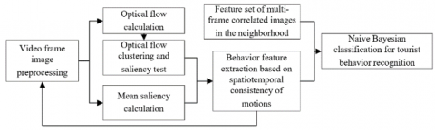
Starting with the spatial retrieval results of the scenic spot, this section presents a tourist behavior recognition method based on spatiotemporal consistency. As shown in Figure 5, the proposed method covers the following steps: the preprocessing of the frame images in surveillance video, the calculation of the tourist motion area, the determination of the size and direction of the tourist optical flow in the frame images based on spatiotemporal consistency, and the naive Bayes classification.
Figure 5. The workflow of tourist behavior recognition based on spatiotemporal consistency
First, the surveillance video of the scenic spot was divided into frames. Each frame image was converted into a grayscale image. Then, the dense optical flow of each image can be calculated by:
$OF\left( p \right)=\psi \left( p \right)x\left( p \right)+\phi \left( p \right)y\left( p \right)$ (26)
where, x(p) and y(p) are the optical flow components of pixel p in the x- and y-directions, respectively; ψ(p) and φ(p) are the coefficients of variation for the two optical flow components, respectively.
The optical flow calculation may be affected by the black areas in the tourist surveillance video. To eliminate the influence, the black areas were subject to the saliency test:
$ST(p)=\left\| {{q}^{*}}-{{q}_{G}}(p) \right\|$ (27)
where, q* is the arithmetic mean of the pixels of the frame images in the RGB color space; qG(p) is the RGB feature of pixel p after Gaussian blurring. It can be seen from formula (27) that the saliency test mainly checks the Euclidean distance between q* and qG(p). The above formula can be normalized by:
$\xi (p)=\frac{S{T}'\left( p \right)}{\upsilon S{{T}_{max}}}$ (28)
where, ST'(p) is the saliency of pixel p after background subtraction; STmax is the maximum saliency in the frame images; υ is a coefficient in the interval of (0, 1). After obtaining the saliency of each pixel, the mean saliency of the pixels in the same optical flow block can be calculated based on the clustering of optical flows:
$\xi \left( b \right)=\frac{1}{{{n}_{b}}}\sum\limits_{i=1}^{{{n}_{b}}}{\xi \left( {{p}_{i}} \right)},{{p}_{i}}\in b$ (29)
where, nb is the number of pixels in optical flow block b. Then, the salient motion area of the frame images can be delineated by:
${{D}_{act}}\left( b \right)=hea\left( p\left( b \right)-\Delta {{\varepsilon }_{\text{1}}} \right)$ (30)
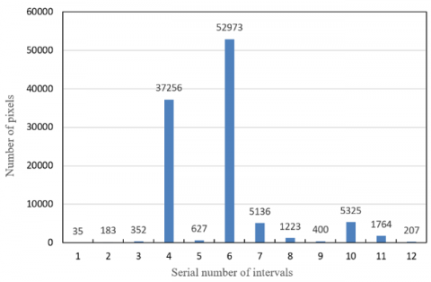
where, hea(⁎) is the optimized Heaviside step function; Δε1 is the ratio of the number of pixels in the target block to the total number of pixels. Next, each optical flow block determined to be processed was subject to feature extraction. After the blocks were clustered by optical flow, the optical flow directions commonly seen in the blocks of the same class were counted (Figure 6), and divided into several histogram intervals. These intervals were sorted in descending order. Let bi be the i-th interval in the ranking. Then, whether an interval should be processed by the histogram can be determined by:
${{D}_{act}}\left( {{b}_{i}} \right)=hea\left( \Delta {{\varepsilon }_{2}}\sum\limits_{j=1}^{K}{{{n}_{{{b}_{j}}}}-\sum\limits_{j=1}^{i-1}{{{n}_{{{b}_{j}}}}}} \right)$ (31)
where, nbj is the number of pixels in interval bj; Δε2 is the ratio of the number of pixels in the target interval to the total number of pixels in the block (hereinafter referred to the interval pixel ratio).
Figure 6. The histogram of optical flow directions
The mean optical flow of block b can be calculated by:
$O{{P}^{*}}\left( b \right)=\sum\limits_{i=1}^{K}{\frac{{{D}_{act}}\left( {{b}_{i}} \right)\cdot {{n}_{{{b}_{i}}}}}{\sum\nolimits_{j=1}^{k}{{{D}_{act}}\left( {{b}_{j}} \right)\cdot {{n}_{{{b}_{j}}}}}}}O{{P}^{*}}\left( {{b}_{i}} \right)$ (32)
where, OP*(b) and OP*(bi) are the mean optical flows of block b and block bi, respectively.
Then, the trend of tourist behaviors can be judged by the optical flow direction derived from the mean optical flows of different intervals. After determining the size and direction of the optical flow in each block, it is possible to recognize the tourist behaviors. Let Ui be the i-th cluster of tourist behaviors. During the motions, the body of a tourist needs to be consistent in space and time. Following this principle, the clustering method can be defined as:
$U\propto \arg \underset{U}{\mathop{\min }}\,\sum\limits_{{{U}_{i}}\subset U}{\left( \sum\limits_{s,t\in {{U}_{i}}}{\left( \begin{align} & \Delta {{\varepsilon }_{\text{3}}}\left\| O{{P}^{*}}\left( {{b}_{s}} \right)-O{{P}^{*}}\left. ({{b}_{t}}) \right\| \right. \\ & +\Delta {{\varepsilon }_{\text{4}}}\left\| u\left( {{b}_{s}} \right)-u\left. \left( {{b}_{t}} \right) \right\| \right. \\ \end{align} \right)} \right)}$ (33)
where, u(bs) is the center coordinates of block bs; Δε3 and Δε4 are adjustment factors for the size and direction of optical flow, respectively. Let r be the search radius. The cluster area being found can be expressed as:
${{{U}'}_{i}}=arg\underset{{{U}_{i}}}{\mathop{min}}\,\left( \Delta {{\varepsilon }_{5}}\left\| \begin{align} & O{{P}^{*}}\left( {{U}_{i}} \right)-O{{P}^{*}}\left. \left( {{U}_{j}} \right) \right\| \\ & +\Delta {{\varepsilon }_{6}}\left\| O{P}'\left( {{U}_{i}} \right)-O{P}'\left. \left( {{U}_{j}} \right) \right\| \right. \\ \end{align} \right. \right)$ (34)
where, Δε5 and Δε6 are adjustment factors for the size and direction of optical flow, respectively. The change of optical flow direction can be determined based on the optical flows of two corresponding sets:
${{T}_{i}}=\left\| O{{P}^{*}}\left( {{U}_{i}} \right)-O{{P}^{*}}\left( {{{{U}'}}_{i}} \right) \right\|$ (35)
where, T=T1, T2, …, TK is the set of displacement features in tourist behavior recognition. To characterize the amplitude of motion, the optical flows F=f1, f2, …, fK were taken as the features of motion amplitude.
Finally, the tourist behavior features were classified by naive Bayesian classification, which can make fast and accurate classification with a few estimation parameters. First, the joint distribution P(Y|T) of output Y and its feature T was searched for:
$P\left( Y\left| T \right. \right)=\frac{P\left( X\left| {{T}_{i}} \right. \right)P\left( {{T}_{i}} \right)}{\sum\limits_{i=1}^{K}{P\left( X\left| T={{T}_{i}} \right. \right)P\left( {{T}_{i}} \right)}}$ (36)
where, the sum of P(Ti) corresponding to all Ti equals 1. Then, the full probability formula for the classification of tourist behavior features was derived by the conditional probability formula.
In order to verify the effectiveness of our method in the retrieval of scenic spot images, 10,583 sub-nodes of the visual words that can quantify the SIFT features were selected to train the standard set of scenic spot images. A total of 25 scenic spot images were chosen as the targets of image retrieval. Each of them has more than 3 correlated images in the image set.
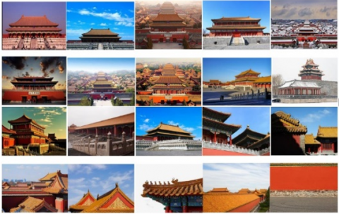
Figure 7 presents the retrieval results of our method on the images of a scenic spot. It can be seen that our method achieved good retrieval effect on the images of prominent buildings in the scenic spot. During the retrieval, the retrieval accuracy of the first 10 correlated images was above 95%, and that of the first 20 correlated images was above 80%.
Figure 7. The first 20 correlated images retrieved by our method
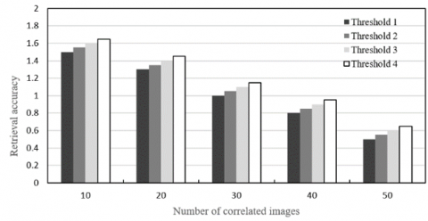
Figure 8. The effects of threshold on retrieval accuracy
To find the multiple correlated images of each target image, the Euclidean distance between global descriptors needs to be compared with the set threshold. This threshold determines the number of correlated images. Figure 8 shows the effects of different thresholds on the retrieval accuracy. It can be seen that the retrieval accuracy and calculation complexity are negatively correlated with the number of correlated images. Hence, the computing load and accuracy should both be considered to configure the accuracy threshold.
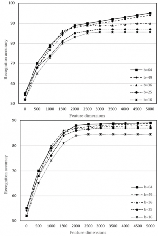
To verify its effectiveness, the proposed method for tourist behavior recognition was tested on a set of surveillance video images containing general behaviors, such as walking, waving, running, and stopping, as well as possible uncivilized behaviors, namely, fighting and defacing. Different numbers of optical flow blocks were arranged in the images of different periods. Figure 9 shows the effects of the number of optical flow blocks on the accuracy of tourist behavior recognition. Obviously, the greater the number of optical flow blocks, the richer the semantic information being mined, and the better the behavior recognition effect.
Figure 9. The effects of the number of optical flow blocks on the accuracy of tourist behavior recognition
Table 1. The recognition accuracies of different methods
|
|
Walking |
Waving |
Running |
Stopping |
Fighting |
Defacing |
|
IM2GPS |
0.727 |
0.678 |
0.714 |
0.679 |
0.674 |
0.749 |
|
SC |
0.819 |
0.710 |
0.832 |
0.762 |
0.735 |
0.809 |
|
QE |
0.831 |
0.811 |
0.846 |
0.781 |
0.807 |
0.838 |
|
SSV |
0.842 |
0.876 |
0.897 |
0.855 |
0.878 |
0.887 |
|
Our method |
0.944 |
0.952 |
0.904 |
0.921 |
0.909 |
0.912 |
Table 2. The recognition accuracies of different methods on different image sets
|
Method |
Dimension |
Behavior recognition accuracy |
|||
|
Image set 1 |
Image set 2 |
Image set 3 |
Image set 3 |
||
|
IM2GPS |
512 |
0.791 |
0.625 |
0.741 |
0.617 |
|
SC |
0.811 |
0.721 |
0.815 |
0.711 |
|
|
QE |
0.825 |
0.812 |
0.836 |
0.801 |
|
|
SSV |
0.877 |
0.856 |
0.889 |
0.842 |
|
|
Our method |
0.921 |
0.910 |
0.932 |
0.901 |
|
|
IM2GPS |
256 |
0.767 |
0.638 |
0.751 |
0.628 |
|
SC |
0.793 |
0.747 |
0.826 |
0.747 |
|
|
QE |
0.815 |
0.854 |
0.847 |
0.827 |
|
|
SSV |
0.823 |
0.878 |
0.899 |
0.857 |
|
|
Our method |
0.896 |
0.925 |
0.936 |
0.922 |
|
|
IM2GPS |
128 |
0.710 |
0.679 |
0.762 |
0.649 |
|
SC |
0.786 |
0.798 |
0.838 |
0.759 |
|
|
QE |
0.801 |
0.886 |
0.855 |
0.831 |
|
|
SSV |
0.835 |
0.898 |
0.901 |
0.868 |
|
|
Our method |
0.842 |
0.947 |
0.941 |
0.937 |
|
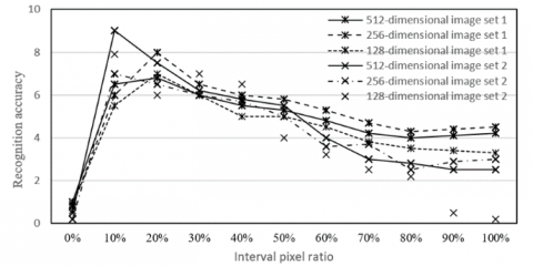
To judge whether an interval needs to be processed by histogram, the number of the intervals to be processed depends on the interval pixel ratio. If the ratio is too small, the extracted image features cannot fully demonstrate the features of tourist behaviors. If the ratio is too large, it is impossible to magnify the salient features that should be highlighted.
Figure 10 compares the effects of the interval pixel ratio on the accuracy of tourist behavior recognition under different image sets of different dimensions. It can be seen that the x- and y- coordinates are positively correlated when the ratio was smaller than 10%, and negatively corelated when the ratio was greater than 10%; the highest recognition accuracy was achieved when the ratio equaled 10%.
To demonstrate its superiority in tourist behavior recognition, the proposed method was compared with IM2GPS, SC, QE, and SSV. The IM2GPS combines global features in traversal retravel; the SC utilizes local features; the QE relies on iterative update; the SSV quantifies the original features based on balanced binary trees.
Table 1 compares the recognition accuracies of different methods on tourist behaviors. It can be seen that our method recognized walking, waving, defacing, and stopping at ultrahigh accuracies. The recognition rates of fighting and running were slightly lower, but better than those of other methods.
Table 2 compares the recognition accuracies of different methods on different image sets. It can be seen that the proposed method outperformed the other methods in the recognition of tourist behaviors on video images of different dimensions. This means the consideration of spatiotemporal consistency can improve the recognition rate of tourist behaviors.
Based on image processing, this paper puts forward a novel method to retrieve scenic spot images and recognize tourist behaviors. Firstly, the authors constructed the framework of scenic spot image retrieval was constructed, and introduced the five steps of extraction of SIFT features: scale space construction, local space extreme point detection, precise positioning of key points, determination of key point size and direction, and generation of SIFT descriptor. Next, multiple correlated images were mined for the target scenic spot image, and the feature matching method between the target image and the set of scenic spot images was explained. Experimental results show that our method achieved good retrieval effect on the images of prominent buildings in the scenic spot. Finally, the authors designed a tourist behavior recognition method based on spatiotemporal consistency. Through experiments, it is learned that our method recognized walking, waving, defacing, and stopping at ultrahigh accuracies, indicating that the consideration of spatiotemporal consistency can improve the recognition rate of tourist behaviors.
This paper is supported by the National Natural Science Foundation of China (Grant No.: 71671054); innovative research project for graduate students of Harbin Commercial University (Grant No.: yjscx2019-560hsd).
[1] Noh, H., Araujo, A., Sim, J., Weyand, T., Han, B. (2017). Large-scale image retrieval with attentive deep local features. In Proceedings of the IEEE International Conference on Computer Vision, pp. 3456-3465. https://doi.org/10.1109/ICCV.2017.374
[2] Hong, R., Li, L., Cai, J., Tao, D., Wang, M., Tian, Q. (2017). Coherent semantic-visual indexing for large-scale image retrieval in the cloud. IEEE Transactions on Image Processing, 26(9): 4128-4138. https://doi.org/10.1109/TIP.2017.2710635
[3] Sabahi, F., Ahmad, M.O., Swamy, M.N.S. (2016). An unsupervised learning based method for content-based image retrieval using Hopfield neural network. In 2016 2nd International Conference of Signal Processing and Intelligent Systems (ICSPIS), pp. 1-5. https://doi.org/10.1109/ICSPIS.2016.7869882
[4] Keni, N.D., Ansari, R.A. (2017). Content based image retrieval for leaf identification using structural features and neural networks. In 2017 4th International Conference on Signal Processing and Integrated Networks (SPIN), pp. 298-303. https://doi.org/10.1109/SPIN.2017.8049963
[5] Radenović, F., Tolias, G., Chum, O. (2018). Fine-tuning CNN image retrieval with no human annotation. IEEE Transactions on Pattern Analysis and Machine Intelligence, 41(7): 1655-1668. https://doi.org/10.1109/TPAMI.2018.2846566
[6] Radenović, F., Iscen, A., Tolias, G., Avrithis, Y., Chum, O. (2018). Revisiting Oxford and Paris: Large-scale image retrieval benchmarking. In Proceedings of the IEEE Conference on Computer Vision and Pattern Recognition, pp. 5706-5715. https://doi.org/10.1109/CVPR.2018.00598
[7] Qi, Y., Song, Y.Z., Zhang, H., Liu, J. (2016). Sketch-based image retrieval via Siamese convolutional neural network. In 2016 IEEE International Conference on Image Processing (ICIP), pp. 2460-2464. https://doi.org/10.1109/ICIP.2016.7532801
[8] Peng, Y.F., Song, X.N., Wu, H., Zi, L.L. (2019). Remote sensing image retrieval combined with deep learning and relevance feedback. Journal of Image and Graphics, 24(3): 420-434.
[9] Li, Z.M., Liu, X.X., Liu, Y.J., Li, H. (2017). Sketch-based image retrieval based on fine-grained feature and deep convolutional neural network. Journal of Image and Graphics, 24(6): 946-955.
[10] Peng, Y.F., Mei, J.Y., Wang, K.X., Zi, L.L., Sang, Y. (2020). Remote sensing image retrieval based on regional attention mechanism. Laser & Optoelectronics Progress, 57(10): 172-180. https://doi.org/10.3788/LOP57.101017
[11] Kaur, M., Sohi, N. (2016). A novel technique for content based image retrieval using color, texture and edge features. In 2016 International Conference on Communication and Electronics Systems (ICCES), pp. 1-7. https://doi.org/10.1109/CESYS.2016.7889955
[12] Srivastava, P., Khare, A. (2016). Content-based image retrieval using scale invariant feature transform and moments. In 2016 IEEE Uttar Pradesh Section International Conference on Electrical, Computer and Electronics Engineering (UPCON), pp. 162-166. https://doi.org/10.1109/UPCON.2016.7894645
[13] Kasban, H., Salama, D.H. (2019). A robust medical image retrieval system based on wavelet optimization and adaptive block truncation coding. Multimedia Tools and Applications, 78(24): 35211-35236. https://doi.org/10.1007/s11042-019-08100-3
[14] Ahmad, J., Muhammad, K., Baik, S.W. (2018). Medical image retrieval with compact binary codes generated in frequency domain using highly reactive convolutional features. Journal of Medical Systems, 42(2): 24. https://doi.org/10.1007/s10916-017-0875-4
[15] Erkut, U., Bostancıoğlu, F., Erten, M., Özbayoğlu, A.M., Solak, E. (2019). HSV color histogram based image retrieval with background elimination. In 2019 1st International Informatics and Software Engineering Conference (UBMYK), pp. 1-5. https://doi.org/10.1109/UBMYK48245.2019.8965513
[16] Hu, H.Y., Zheng, W.F., Zhang, X., Zhang, X., Liu, J., Hu, W.L., Duan, H.L., Si, J.M. (2020). Content-based gastric image retrieval using convolutional neural networks. International Journal of Imaging Systems and Technology. https://doi.org/10.1002/ima.22470
[17] Liu, J.W. (2018). Research on LSTM behavior recognition method based on extended data set. Liaoning University.
[18] Ma, Y.X., Tan, L., Dong, X., Yu, C.Z. (2019). Behavior recognition for intelligent surveillance. Journal of Image and Graphics, 24(2): 282-290.
[19] Luo, F.B., Wang, P., Liang, S.Y., Xu, G.F., Wang, W. (2019). Anomalous behavior recognition based on deep learning and sparse optical flow. Computer Engineering, 46(4): 287-293, 300. https://doi.org/10.19678/j.issn.1000-3428.0054605
[20] Mabrouk, A.B., Zagrouba, E. (2018). Abnormal behavior recognition for intelligent video surveillance systems: A review. Expert Systems with Applications, 91: 480-491. https://doi.org/10.1016/j.eswa.2017.09.029
[21] Yousefi, S., Narui, H., Dayal, S., Ermon, S., Valaee, S. (2017). A survey on behavior recognition using wifi channel state information. IEEE Communications Magazine, 55(10): 98-104. https://doi.org/10.1109/MCOM.2017.1700082
[22] Batchuluun, G., Kim, J.H., Hong, H.G., Kang, J.K., Park, K.R. (2017). Fuzzy system based human behavior recognition by combining behavior prediction and recognition. Expert Systems with Applications, 81: 108-133. https://doi.org/10.1016/j.eswa.2017.03.052
[23] Haataja, E., Malmberg, J., Järvelä, S. (2018). Monitoring in collaborative learning: Co-occurrence of observed behavior and physiological synchrony explored. Computers in Human Behavior, 87: 337-347. https://doi.org/10.1016/j.chb.2018.06.007
[24] Ahmad, J., Muhammad, K., Lee, M.Y., Baik, S.W. (2017). Endoscopic image classification and retrieval using clustered convolutional features. Journal of Medical Systems, 41(12): 196. https://doi.org/10.1007/s10916-017-0836-y