Pooja Satish* | Mallikarjunaswamy Srikantaswamy | Nataraj Kanathur Ramaswamy
© 2020 IIETA. This article is published by IIETA and is licensed under the CC BY 4.0 license (http://creativecommons.org/licenses/by/4.0/).
OPEN ACCESS
Image Deblurring is a very popular area of research in all over the world. It is an illposed problem which still does not have an ideal solution. Therefore, in order to analyse the research problems and to understand the statement of image deblurring we look in to the state-of-the-art methods proposed in various recent publications. Hence, the present study is focused on the overall review of the techniques used in image deblurring and their solutions to tackle the illposed problem using mathematical model. Based on the overall technique simple MAP model falls short in either deriving accurate convergence to the global optimum or computational implementation. Convergence of the algorithm is the most important factor for the effective performance of Lo and L1 norms for regularizers for theoretical applications. The importance of the choice of the correct estimator and the role of various priors in solving the imaging inverse problem using the MAP estimation method is discussed. The consequence of different priors to the rate of convergence of the MAP algorithm and its computational complexity are studied and tabulated.
blind deconvolution, Maximum A Posteriori Estimation (MAP)
The process of image capture is not perfect and even under best conditions the captured image is prone to degradations. The degradations so caused are due to two main factors one is noise which is random in nature and the other is blur which is deterministic in nature. Image deblurring is the process of retrieving the latent sharp image from a captured blurry and noisy image. Image deblurring has various applications such as in astronomical images, remote sensing, CCTV footage, medical images, or in onetime occurring situations where multiple images of the same cannot be captured. Degradations are unavoidable in such images due to various factors. Such as regulated intensity as in medical imaging where the intensity levels of the incident rays of an X-ray, CT or MRI machine is maintained at a regulated level to avoid damage to the human organs; or continuously changing atmosphere, light and refraction conditions of astronomical images. Also, degradations are caused due to imperfections in the optics used such as a camera lens or the lens of a microscope used to magnify objects under inspection and relative motion between the imaging scene and the camera.
This paper is a comprehensive survey of the different Image deblurring techniques. We analyze the strengths and weaknesses of different image deblurring algorithms.
Many papers on image deblurring have been presented in recent times. Despite various publications none of them have been able to achieve an ideal solution to the illposed problem. This paper takes a fresh approach to tackling the problem, instead of proposing an improvement on the existing methods, we aim at understanding the concept of image deblurring first. Hence, we start from understanding the blurring of images during the image formation, and further go on to analyze the different methods designed to solve this problem statement, their advantages and disadvantages. This research is aimed at understanding the fundamentals of image deblurring. This paper is divided into various sections. Section II gives insight into mathematical model for image formation and further discusses in detail the mathematical model for image deblurring which is necessary to solve the image deblurring problem statement and its few variations seen in literature. Section III reviews the different methods used in solving this ill-conditioned problem statement. Section IV gives a detailed description of the mathematical model of the Maximum A Posteriori (MAP) Estimation technique. In section V the different additions and improvements proposed for the simple MAP model in recent literature are shown and their effect on the MAP algorithm is analyzed. Section VI shows the results of the experiments on the simple MAP model. The main contributions of this paper are it compares and analyses the different methods used for image deblurring.
Image Deblurring is an imaging inverse problem. In order to solve an imaging inverse problem, the process that occurs when a scene is sensed by the image sensors and converted into an image has to be inversed to recover the objects that constitute the image of the scene. The process of sensing the light, both incident and reflected from the objects of a scene and converting this sensed component of light into image components is mathematically represented as integration as shown by Ribes and Schmitt [1]. Now to retrieve the scene elements from a captured image requires inversing this integration process. The integral process of image capture is represented by the Eq. (1). Where g(x) is the function representing the captured image, φ (x, λ) and o (λ) represents the integral kernel which varies physically depending on the operation and the property of the object we are measuring respectively. The noise component which is inevitable during acquisition is represented by n(x).
$g(x)=\int_{\gamma}^{\rho} \varphi(x, \lambda) o(\lambda) d \lambda+n(x)$ (1)
The continuous functions in the above equation have to be discretized in order to solve the equation numerically. The discretized form of Eq. (1) is given by g = hO+n, where g, o, and n represent the vectors of the acquired image, the property of the object and the additive white Gaussian noise respectively. The term h is the matrix representing the kernel of the application.
The obtained image is a two-dimensional function and can be inversed using various methods, such as Fourier Transform method, regularization, interpolation method, direct and indirect reconstruction methods. Now to represent the mathematical model of image deblurring we assume the degradations that cause blurring in an image are linear and position invariant [2]. This problem is further complicated with the inevitable addition of noise n. The degraded & noisy image g is represented by the Eq. (2) where $\otimes$ represents 2D convolution and + depicts addition of the white Gaussian noise n. Assuming the degradations on the image are linear are space invariant it can be represented mathematically as convolution of the degradation function h and the unknown sharp image o. The blurring of an image during image formation is depicted in Figure 1.
Figure 1. Block diagram representation of the problem statement
$g(x, y)=h(x, y) \otimes o(x, y)+n(x, y)$ (2)
Hence recovery of the sharp 2D image requires a 2D deconvolution process. The recovery of the sharp image from just the captured image and with no knowledge of the sharp image and the degradation function is known as Blind Image Deconvolution. It consists of only one known component that is the degraded & noisy image g. Hence the problem is severely illposed as defined by Hadamard [3], i.e. its solution is not unique and small changes to input data (degraded image g) lead to large variations in output (latent original image o). Since the problem statement in the Eq. (2) is an inverse problem and inverse problems are already illposed due to data deficiency, the problem statement is an inverse, ill-posed problem statement. The Eq. (2). estimates the point spread function of the captured image for a space invariant assumption. But Šroubek et al. [4] show that blurring is a space variant phenomenon, in such a situation the expression in Eq. (2) has to be modified to accommodate the change in the blur kernel of the captured image as a function of its position.
Deconvolution with a known degradation function h and a known degraded image g is called as Non-Blind Deconvolution. Here considering only the degradation and ignoring the noise affecting the image and discretizing the problem statement shown the Eq. (2) reduces to g = h$\otimes$o, which has two known values and just one unknown. Schneider et al. [5] present a benchmark to compare non-blind deconvolution algorithms. This gives an insight into various image de-blurring methods and their use in the automated visual inspection systems. Kotera et al. [6] solve the blind deconvolution problem using only a single channel of observation, this is also called as a single channel blind deconvolution (SCBD) problem. While Šroubek and Milanfar [7] use multiple channels of observation in an alternating minimization algorithm using MAP Estimation to derive the sharp image, this is known as a multi-channel blind deconvolution (MCBD) where channel of observation represents the observed degraded image which is required to be deblurred. Hence single channel blind deconvolution represents a single observed degraded image. Whereas, in multi-channel blind deconvolution represents multiple observations or multiple degraded images of the same scene. Delbracio and Sapiro [8] use a burst of images, which consists of multiple images captured sequentially by the camera. Fourier transformation is used on the accumulated burst along with blur kernel to derive the sharp image in the Fourier domain. MCBD offers more prior information about the original image which tends to reduce the ill-posedness of the problem statement to some extent.
The Blind image deconvolution problem is solved using different approaches by different researchers in various publications. Some of the methods of blur kernel estimation in literature include restoration through filtering methods for example Giannakis and Heath [9] design a series of linear FIR filters which are used in a MCBD problem statement to directly derive the restored image and a subsequent set of FIR filters for blur identification. Hosseini and Plataniotis [10] propose a convolutional filtering method using Finite Impulse Response filters.
This section gives a general insight into the different methods used for image deblurring described in literature and their mathematical models. This gives an understanding of the representation of images in different mathematical models and their manipulation to derive deblurred images in the various methods.
3.1 Linear model theory
In the Linear Model Theory, degradation of an image is understood as conversion of sharp edges in it into blurred ones, this process is assumed to be linear and the supposition is that, the blur is the most significant part of this procedure. The initial sharp image and the captured degraded images are considered to be digital grayscale images. A blur is the easiest form of degradation. For the purpose of mathematical implementation of the linear model, both the input blur image and resulting sharp image are assumed to be matrices of size (m x n) and the degrading of columns is executed autonomously of the degrading of rows. The matrix Ac with size m x m and Ar with size n x n are used to denote this autonomous blurring. The relation between the latent (sharp) and the captured (degraded) images are shown in Eq. (3)
$G=A_{c} O A_{r}^{T}$ (3)
where, the term Ac O denotes the blurring of every column in image O & O ATr denotes the blurring of every row in image O and G denotes the degraded blurry image. In order to derive the sharp image, O the expression in Eq. (3) is rewritten to derive O as shown in Eq. (4) below
$O=A_{c}^{-1} G\left(A_{r}^{T}\right)^{-1}$ (4)
But this resulting image O does not mirror the initial sharp one due to the exclusion of noise at the time of taking the picture. Noise in an image is originated by irregularity and a variety of imperfections in the imaging gadgets, such as lens imperfections etc. Hence, unessential and false data is added with the captured image. In order to address this, we include the noise term in our model. Hence by including the additive noise in the Eq. (3), the expression representing the model for the blurred image changes to the one shown in Eq. (5).
$G=A_{c} O A_{r}^{T}+E$ (5)
In the above equation, the noise in the image is represented by the matrix E of size m x n. From this the sharp latent image can be computed by using the expression shown in Eq. (6).
$O=A_{c}^{-1} G\left(A_{r}^{T}\right)^{-1}-A A_{c}^{-1} G\left(A_{r}^{T}\right)^{-1}$ (6)
The second term on the RHS denotes the noise inverse term. From the above expression we can infer that image reconstruction using this model leads to the dominance of the inverse noise term in the resulting degraded image. Faramarzi et al. [11] design a unified method which performs both single image blur deconvolution and multi-image super resolution. Deblurring or blur deconvolution can be thought of a special case of blind super-resolution with a magnification factor of 1. Here a linear forward imaging model is used to derive low resolution images from a high resolution captured blurred image. The noise factor in these low resolution images are assumed to be the same. Since the noise is same in all the LR images the blur can be rectified by using non uniform interpolation. The pixel values of the new high-resolution image are computed from the LR images using either linear, cubic, or spline interpolation schemes.
3.2 Singular value decomposition method
In the Singular Value Decomposition method of deblurring the problem statement is solved for by finding the SVD. This is a more obvious model, as per this model the procedure of blurring is carried out on rows and columns of image at the same time. In the beginning the sharp image I and the degraded image G will be normalized by modifying the size of G & I to a predefined size of N=m x n. This normalization is necessary to maintain uniformity of results with input images of varying sizes. The vectors thus formed are Iv which represents the sharp image and Gv is the vector representing the blurry and noisy image, the vector Ev represents the additive noise and the relation among the vectors is given by the Eq. (7)
$G_{v}=A I_{v}+E_{v}$ (7)
Here it is implied that A is the known degradation matrix of size N x N, which is estimated by the imaging system. The term Ev denotes the noise vector. Therefore, the sharp image reconstruction is given by the Eq. (8)
$I_{v}=A^{-1} G_{v}-A^{-1} E_{v}$ (8)
In the above equation, the inverse term indicates the inverse of the degradation function. If the effect of the inverse degradation function and noise are more on reconstructed image, the images which are reconstructed would turn more distorted. Hence by utilizing the SVD (singular value decomposition) on the degradation function A, we derive two orthogonal matrices U and V given by the equation $A=U \Sigma V^{T}$ by using this in the Eq. (8) the effect of the inverse noise terms on the reconstructed images can be reduced to particular cases only, such as when the singular values decay to a value close to zero or when the error components are small and have approximately same magnitude for all v.
3.3 Richardson-Lucy deconvolution Algorithm
The Richardson-Lucy deconvolution Algorithm is also called as Lucy Richardson Algorithm is a methodology utilized to regenerate the sharp image from the degraded images. Where the blurring is caused by a known PSF (point spread function). Hence the deconvolution method presented by Richardson and Lucy is a Non-Blind Deconvolution. The main idea of this algorithm is to represent the known degraded image pixels with respect to the unknown sharp image and the known PSF. The mathematical relation between the degradation function H, the degraded image g & the sharp image f are described in Eq. (9) and (10).
$H f=g$ (9)
$\sum_{j} h_{i j} f_{j}=g_{i}$ (10)
where, $h_{i j} \geq 0, f_{j}>0, g_{i}>0$ and $\Sigma_{j} h_{i j} f_{j}=1, \Sigma_{j} f_{j}=\Sigma_{j} f g_{j}=N$ and $h_{i j}, f_{j}, g_{j}$ are considered as probability density functions. The algorithm exploits the relationship between the variables in the Eq. (10) to derive and find a probabilistic solution for the unknown sharp image, Hence the estimated sharp image using the RLA is given by the Eq. (11)
$f^{n+1}=f^{n} H\left(\frac{g}{h f^{n}}\right)$ (11)
The main advantage of this algorithm is that it does not require any prior information from the input image and is sufficiently effective even in the presence of noise. But the noise increases as the number of iterations increases. RLA is a popular algorithm in image deblurring with many different researchers designing a new blind deconvolution algorithm based on the Richardson-Lucy Algorithm. Many modified versions of the RLA are seen [12]. The RLD algorithm is also used as the subsequent non blind deconvolution method in many recent image deblurring researches where a new method for PSF estimation is designed [13]. Further Anacona-Mosquera et al. [14] design a hardware implementation for the RLA algorithm in an FPGA- based platform using filters or masks to perform the convolution operation. The dot products in the Eq. (11) becomes convolution operators in the spatial domain. Masks can be designed to perform any filtering operation such as smoothing, edge detection, etc. The hardware architecture of the RLA and the convolution filtering operation using masks is described.
3.4 Neural networks for image deblurring
For a Neural network method first a scheme for deblurring is built using a set of blurred images and their corresponding sharp images. Initially the system is fed by blur and their corresponding sharp images. This kind of training activates the system to guess the sharp image related to the blur images. Several neural networks supported methods are utilized in literature, such as by Schuler et al. [15]. The algorithms used for the neural node or network training may vary depending upon the requirements of the algorithm, for example a simple LMS (Least Mean Square) is used to predict true pixels to regenerate degraded images this forms a purely founded from of neural network. Similarly, another algorithm which is based on gradient decent and back propagation in a web consisting of 3 layers of neural nodes is used for image restoration [11]. This non collinear propagation utilized to restore images is unsuccessful in generating a full quality restored image. This algorithm also has a large scope for improvement in increased speed and reduced complexity of calculation since there is very little quantity of utilized neurons in this technique of training. Hence to improve this back-propagation method the neural nodes are designed based on the Artificial Bees Colony Algorithm. The ABC algorithm works by finding the global best solution for a given criteria. In the algorithm the neural nodes imitate a swarm of bees locating food. The ABC algorithm is applied to both image enhancement and edge detection steps of image deblurring.
3.5 Parametric PSF estimation methods
Parametric estimation methods are where a parametric mathematical model for deblurring is used to solve for the true blur kernel and the sharp image. Xue and Blu [16] design a parametric PSF estimation method using Stein’s unbiased risk estimate for MSE. The parametric equation is designed in the frequency domain and a minimization algorithm is formulated to estimate the PSF. The estimated PSF is then used in a non-blind deconvolution algorithm to derive the sharp image.
Shah and Dalal [17] propose a parametric PSF estimation technique in the Cepstrum Domain, which estimates the motion blur parameters such as length and angle. The parametric methods are challenging as they do not have prior information available for PSF estimation. They use a method based on spectral or cepstral zeroes. The major difficulty of solving problems in the spectral domain is that the image frequency components and the blur frequency components are mixed together which reduces the efficiency of PSF estimation. The Cepstrum is derived by taking the Fourier Transform of the log magnitude of the blurred image. To avoid the noise components the range of the cepstral components which is dynamic is reduced by taking the Log of its absolute value, this gives the modified cepstrum. Radon Transform is used on the modified cepstrum to find the direction of motion. The maximum value of the radon transform is subtracted with 90° to derive the major direction of motion blur. The blur length is calculated from the rescaled and modified cepstrum with the help of an algorithm designed specifically to calculate the difference between the central peak and side peaks.
3.6 Iterative methods
The Iterative methods seen in literature utilize the iterative rebuilding of linear blurs in images brought about by point-wise non linearity. It is represented that the repetitive deconvolution techniques can utilize different sorts of an earlier information about the class of accomplishable results to expel non-moving foggy spots. They clarify the issue of convergence to relate and think about surely understood algorithms, for example, Wiener filters, constrained least square and inverse filters which are demonstrated to restrict arrangements of varieties of the iterations [18]. At last the regularization term is used in the algorithm to restrict the permitted furthest reaches of noise amplification brought about by the inverse nature of the problem statement, for example, deconvolution issues in addition the impact of noise can be ended after various limited iterations. General class of iteration shrinkage threshold algorithm (ISTA) are used to clear the issues of linear inverse problems which happens in image processing. These methods are popular due to their ease of computational application however it is known that the convergence is moderate. Hence the FISTA (Fast iterative threshold algorithm) was introduced to increase convergence speed while retaining the ease of computation of algorithm of ISTA this has increased the convergence rates to that of average of the state-of-the-art methods.
3.7 Stochastic model
Stochastic models are based on the analysis of the probability density function of the input blurred image. Xiao et al. [19] design a blind image deblurring algorithm called as the Stochastic Random Walk Optimization Algorithm which is based on a simple random search technique. In this algorithm local solution updates are derived from a random walk chain at each pixel location in the captured deblurred image, these updates are verified against an objective which checks for the energy quantum and decides whether to add or remove it into the final estimate of the PSF. This algorithm iterates between the above algorithm for accurate PSF estimation and a non-blind deconvolution algorithm to derive the corresponding sharp image. The non-blind deconvolution algorithm used is from their previous work [20] which is focused on a stochastic framework for efficient non-blind deconvolution. The highlight of this algorithm is its simplicity in solving the complex imaging inverse problem. It can easily handle priors without the need for changing the already complex mathematical model to accommodate the necessary priors to regularize the expected solution, which further leads to the complication of too many unknowns.
3.8 Deblurring based on the probabilistic Bayes model
The two most popular methods of image deblurring are based on the Bayesian Framework of estimating the posterior distribution using its relationship with the likelihood function and the prior distributions. This relationship is shown in the Eq. (12), where $p(o, h \mid g)$ represents the posterior distribution of the image which is proportional to the likelihood function given by $p(g \mid o, h)$ and the priors on the image and the blur kernel $p(o) p(h)$ respectively.
$p(o, h \mid g)=\frac{p(g \mid o, g) p(o) p(h)}{p(g)} \alpha p(g \mid o, h) p(o) p(h)$ (12)
The first method based on the probabilistic Bayes model is the Variational Bayes method [21, 22], which estimates the mean posteriori values. This method is effective in accurate PSF estimation for various types of blurs such as motion blur, out-of-focus blur in various images, but solving the Bayes formula requires approximation of integration, which fails in computational implementation. Hence, we can infer that hardware implementation of Variational Bayes method is not a practical option. MAP estimation method is the most popular method used to solve the problem statement, due to its ease of numerical implementation. The MAP estimate is based on the rationale that the optimum value of the logarithm of a function is the optimum value of the original function, as the logarithm is a monotonic function. Many researchers have used additions to a simple MAP model to derive better results. The MAP estimation method and its variants provides for ready computational implementation. The next section gives a brief understanding of the mathematical MAP model and its types.
3.9 MAP estimation
The Maximum a Posteriori Estimation is a probabilistic model used to solve the Eq. (2). This is probably the most used method for image deblurring by researchers, probably because of the versatility it offers in its implementation. The MAP model can be designed to use any prior on the image or on the PSF at various stages of the algorithm. We observe that this method can be applied to deconvolve a blurred image in two ways. One is through the simultaneous estimation of the PSF and the sharp image as shown by Šroubek and Milanfar [7] where they use alternating minimization algorithm for the simultaneous estimation of the sharp image o and its blur function h. The other method is through the initial estimation of the PSF and the subsequent non blind deconvolution to restore the image [23]. Traditionally non blind image deconvolution is called the classical image deconvolution. There are various classical deconvolution algorithms such as the Richardson-Lucy algorithm [14] which can be used to deblur the image once the blur function h is derived using MAP estimation. The MAP estimation for deconvolution was previously presumed to derive a trivial delta kernel solution only, but recent improvements have shown that the MAP method of estimation can derive effective results even for a non-trivial blur kernel [15, 24, 25] etc. The severely ill posed problem of blind image deconvolution is converted into a mathematically solvable problem statement using a MAP estimate or Maximum a Posteriori estimate. A MAP estimation is similar to maximum likelihood estimation where the unknown data is estimated using the known experimental data. This is done through maximizing the posterior distribution. The MAP estimation can be executed in two ways which is described below.
3.9.1 MAPh,o
This is the simultaneous estimation of both the blurkernel h and the sharp image o
$\max _{h, o} \operatorname{Pr}(o, h \mid g) \propto \max _{h, o} \operatorname{Pr}(g \mid o, h) \operatorname{Pr}(o) \operatorname{Pr}(h)$ (13)
The second term on the RHS of Eq. (13) is the maximum likelihood term, Pr(o), Pr(h) are the priors on the image o and the blur kernel h. This is represented as a minimization expression where the MAP approach seeks new values for h & o by minimizing the below expression
$(\hat{h}, \hat{o})=\min _{h o} \lambda\|(h \otimes o-g)\|^{2}+\sum_{i}\left|k_{x, i}(o)\right|^{a}+\sum_{i}\left|k_{y, i}(o)\right|^{a}$ (14)
where, $\lambda\|(h \otimes o-g)\|^{2}$ is the data fitting term derived from the logarithmic function of the maximum likelihood term i.e., the second term on the RHS of the Eq. (14). Since algorithm is the optimal value of o in the original function. The terms $\left|k_{x, i}(o)\right|^{\alpha} \&\left|k_{y, i}(o)\right|^{\alpha}$ represent the horizontal and vertical derivatives of the pixel i in the image o. Here the data fitting term is constant and the prior varies. Varying the exponential term α gives different priors that are assumed on the image o. For instance, α valueless than1 leads to sparse priors, α value of 1 leads to a Laplacian prior, and α value of 2 leads to a Gaussian prior. Natural images are in the range of α[0.5,0.8]. Different types of priors are successful for different types of images, for step edges as parse prior gives a correct sharp image while a Gaussian prior gives a blurry explanation, for an arrow peak, low values of α are preferred. Natural images contain more medium and narrow peaks than step edges hence sparse priors are also inefficient. Apart from the selection of priors we also note that as the size of the image window is increased the blurry result is preferred, whereas near significant edges the sharp image results. This can be explained as the blur has two opposite effects on the image likelihood, near significant edges it induces sparsity and decreases likelihood, whereas in natural images it reduces the derivatives variance and hence increases its likelihood. We can observe that for a simultaneous recovery of both the sharp image o and blur kernel h using a MAP estimation the result is dominated by the edges. This problem persists even when an exact prior is chosen in natural images and a very large number of measurements are taken.
3.9.2 MAPh
The draw back in MAPh,o is addressed by estimating just the blur kernel instead of simultaneous estimation. This leads to the second method of MAP, i.e. MAPh. In the MAPh method the blur kernel h is estimated and non-blind deconvolution is used to recover the sharp image o. We have seen that MAPh,o fails to acquire quality measurements even with very large number of measurements. Hence in order to increase the measurements we take into consideration the strong asymmetry of the dimensions of the unknowns h and o. While o increases with image size h is a constant value and is small in size and given in Eq. (15) and (16)
$\hat{\mathrm{h}}=\arg \min _{h} p(g \mid h) p(h) / p(g)$ (15)
where,
$p(g|h)=\int{\exp }-\frac{1}{2{{\eta }^{2}}}||({{h}_{o}}-g)|{{|}^{2}}-\frac{{{\alpha }^{2}}}{2{{\alpha }^{2}}}dx$ (16)
3.9.3 The MAP Algorithm
The MAP Algorithm is implemented in frequency domain to reduce the time taken for the complicated deconvolution process in the time domain. Hence the first step is to convert the input image data into frequency domain using Fourier Transformations. Next the Maximum A Posteriori (MAP) estimate of the problem statement is divided into o - step estimate and h - step estimate. The priors for each step are chosen and are integrated into the mathematical formula. The alternating minimization algorithm is used to alternatingly minimize o and h to the global minimum or the global optimum. Each minimization problem in the o - step and the h- step is solved using Augmented Lagrangian Methods (ALM). Alternating Minimization is continued until convergence. When the convergence point is reached, estimated PSF h and sharp image o are obtained. The main requirement of the algorithm here is to achieve this convergence at the true minimum. Perrone and Favaro [26] shed light onto the workings of the simple MAP model. They shred the MAP estimation from all its recent additions and show that the most important factor while implementing the maximum a posteriori algorithm is in the careful attention to details during its execution. They design a new alternating minimization algorithm, known as the Projected Alternating Minimization (PAM) algorithm, which is designed to include these details during execution such as the initial assumption of a delta kernel which gives better blur prediction and including priors on the kernel in a later stage to refine the final estimated PSF. They confirm that using a maximum a priori in the both sharp image and the blur leads to the selection of local minima hence to derive a correct solution simultaneous minimization of both the sharp image and the blur is not used in the PAM algorithm. Another variation to the existing Alternating Minimization algorithm is shown by Padcharoen et al. [27] where an accelerated alternating minimization algorithm (AAMA) is proposed, which uses a technique called the Accelerated Proximal Gradient (APG) method to increase the convergence speed of the usually slow gradient descent method.
Even a classical deconvolution problem with only one unknown is ill-posed. One popular method of solving this kind problem is by using priors on the image. Šroubek et al. [28] show that a prior is a set of information about the image that is assumed before processing it. The information could be any known value about the image, such as the colours in it or a distribution it follows [29]. This known information is incorporated in the processing such that it leads to the algorithm choosing the correct image. Some effective additions and variations to the simple MAP model seen in literature are mentioned below.
4.1 Regularization
Regularization is a technique of introducing an additional term to solve an inverse ill posed problem. A regularization term chosen can be bounds on the vector space norm, or a data fitting term restricting the smoothness of a function; it is used to force the values to a predetermined set. A Regularization term is added to a loss function, the most commonly used optimization formula is given in Eq. (17):
$\min _{o}=\frac{1}{2}\|(o-g)\|_{2}^{2}+\frac{\lambda}{2} \phi(\mathrm{x})$ (17)
where, o and g are the sharp and the captured degraded images respectively, ϕ (x) is a non-convex regularizer, λ > 0 is the regularization parameter. The regularizer term varies according to the regularization method opted, for example in case of the widely used Lp norm regularization the regularizer term is as shown in the expression below, The Lp norm is the most often used regularization term in MAP estimation for image deblurring The Lp norm is a non-convex regularizer and is given in Eq. (18)
$\phi(x)=\left(\sum_{i}\left|x_{i}\right|^{p}\right)^{\frac{1}{p}}$ (18)
The Lo norm introduces a sparsity constraint to the objective function. It can be defined as the number of non-zero elements in the function [30]. But since solving the Lo norm is an NP hard problem it will be difficult to solve it. Xu et al. [31] propose a sound mathematical model to implement Lo norm. This induces sparsity and derives state of the art deblurring results. Zhang and Kingsbury [32] use a majorization-minimization approach to a fast Lo based image deconvolution with variational Bayesian inference. Here the Lo norm is approximated by iteratively reweighing the L2 norm, deconvolution is wavelet based. Another feasible option is the L1 norm also called as LASSO which is a convex regularizer used by Xu and Jia [33] to design a method of kernel estimation consisting of two phases, one to initialize the kernel and the other to refine it. Lin et al. [34] design a hybrid L1 - L2technique based on Huang et al. [35], where variable splitting is incorporated to solve the optimization problem. The regularization problem is divided into three sub problems applying a different technique for each sub problem the three sub problems are PSF estimation, image restoration for which Tikhnov regularization is used and an image denoising problem optimized using TV regularization. Krishnan et al. [36] use a ratio of L1/ L2 norm to induce sparsity. As reducing the L1 norm on high frequencies leads to denoising on one hand and results in a blurry image on other hand. Hence L1 / L2 acts a normalized version of the L1 norm and performs well for blur present in natural images. Optimizing the L1 / L2 norm leads to the accurate PSF which is used in a non-blind deconvolution algorithm designed by them [37], which they claim to derive better results than RLA for non-blind deconvolution, to result in the latent sharp image. Li et al. [38] show that the edge details could possibly be damaged by using Hyper-Laplacian priors and propose a regional division method which can preserve edge details and avoid the ringing artefacts. Here the weighing term which controls the regularization factor on the image pixels is used to steer the result to preserve edges. A weighing term of larger magnitude preserves the image details whereas a smaller value of the weighing term reduces the ringing artefacts. Hence by adaptively varying the magnitude of the weighing terms according to the region of the image, the Hyper-Laplacian priors can be steered to retain image edges as well as reduce ringing artefacts. Chen et al. [39] present a simulation study of using different regularization parameters in a L2 norm regularization model. The numerical results of eight different regularization parameters are compared for an input ultra sound image. Portilla et al. [40] use L2 norm to convert the Lonorm into a computationally implementable format.
Another significant regularization technique is the anisotropic diffusion [41] (also called Perona and Mallik diffusion) where an image is restored preserving its details. This method is also adopted by You and Kaveh [42]. Here spatial correlation of the image pixels is exploited. The solution here is mainly focused on Shift-Variant blur. The authors point out the drawback of using existing techniques such as a shifting window Kalmann filter for a shift-variant PSF. The anisotropic regularization technique is first applied to shift invariantly blurred images. This is further adapted to shift variant blurred images. Chan and Wong [43] original TV, follow the same approach but use TV (Total Variation) Regularization. The TV norm for regularization is extremely effective for recovering edges of images and also in some blurs such as out-of-focus blur or motion blur [44]. This is implemented in an alternating minimization algorithm. This is an iterative algorithm that gives effective deblurred results in a few iterations. Once the input function is regularized the main objective now is to solve the MAP model of this regularized function such that it converges effectively to a global minimum. Augmented Lagrangian Multiplier (ALM) methods along with Split Bergman Iterations are used to solve the regularized MAP model as shown by Kotera and Šroubek [6]. A TV algorithm based on split Bregman iterations with adaptive weights is shown by Chen [45] the weight for every parameter is based on the property of every pixel. The higher order partial derivatives of every pixel are used for this. Split Bregman iteration is used to solve the blind deblurring L1 problem.
The ALM method is proven to converge even with a non-convex objective. As converging is of prime importance in optimizing the solution, regularizers such as Lp norm go hand in hand with algorithms such as ALM, Alternating direction method Multipliers (ADMM), Split Augmented Lagrangian and Shrinkage Algorithm (SALSA). Wang et al. [13] design a new half quadratic model which they claim to be the first half quadratic mathematical model for the isotropic TV/ L2 used to solve the blind deconvolution problem statement. Its subsequent algorithm leads to the new alternating minimization algorithm which can be implemented on both grayscale and RGB images. This algorithm FTVd allows the utilization of fast transforms in quadratic minimization. They show strong convergence results. For a fixed β they prove their half quadratic model converges to a solution then by using the finite convergence property they show that their model converges with q-linearity which can also be said to be quadratic convergence rate, by which the half quadratic model converges. They experimentally test the convergence rates for different values of βon a set images with synthetic blur. They further derive an optimal numerical value for β and compare the performance of their algorithm with similar state of the art algorithms and show that their algorithm improves the speed of execution of an TV/ L2 model thus putting it on par with other widely used models in image deblurring.
The regularizers are the priors which when applied on the simple MAP estimation model shown in Eq. (14), it forcefully steers the resulting sharp image and the estimated PSF in particular direction. For example, Lo norm enforces sparsity which is a very desirable property for a prior on the MAP algorithm, but solving the Lo norm regularizer is classified as an NP-Hard problem. But due to its very desirable property of inducing sparsity it has been used in conjunction with L1 norm and L2 norm as seen in L2 – Relaxed L0 pseudo norm and L1 – Relaxed L0 norm. The main aim of this is to relax the NP-Hard nature of the Lo norm. Though these conjunctions have managed to incorporate the advantages of the Lo norm they have severe shortcomings. In case of the L1–Relaxed L0 norm Gradient descent which is a popular method for deriving the global optimum cannot be applied. As the gradient descent requires the function to be differentiable at 0 and the L1 norm is not differentiable at 0. Similarly, the main advantages and disadvantages of the various regularizers are tabulated in Table 1.
4.2 Edge detection techniques
Edges in an image are distinguished as the begin or end of a homogeneous region of the image for example the boundary of an object in an image forms an edge in the image as the pixels constituting the object vary significantly from the pixels of the background. All the pixels of the same object form a region, as all these pixels depict a similarity either in colour, texture or amplitude. The pixels which form the boundary of an object have neighbouring pixels which do not have this similarity trait specific to the region.
Detecting the edges of an image is a definite way of sharpening a blurry image. The edges in an image can be calculated by the gradient vector. The edges in the images can be used as a prior in the MAP estimation, as shown in the Figure 2. Shrivakshan and Chandrasekar [46] list and compare the results of various edge filters on a test image. Sobel, Prewitt and Roberts operators for edge filtering is used exhaustively in numerous image processing papers for various applications. Finding zero crossings of the second derivative is another popular approach.
$(\hat{h}, \hat{o})=\min _{h, 0} \lambda\|o-g\|^{2}+\sum_{i} w_{i}\left|k_{x, i}(o)\right|^{\alpha}+\sum_{i} w_{i}\left|k_{y, i}(o)\right|^{\alpha}$ (19)
Edge reweighing [23] is implemented on a simple MAP estimation using the Eq. (19) shown above. Edge detectors and operators such as Sobel, Prewitt etc. are used to reweigh the gradients. The non-uniform weights $w_{i}$ prevents the delta solution, by increasing the smoothness penalty on low contrast regions of the image. Also, the likelihood weight λ is updated after each iteration. Choosing the likelihood weight from a low value to a high value helps in deriving the true blur solution, as a low λ is most likely to pick the true blur in the initial iterations it is important to have a low λ during the initial iterations. It is noticed that recent papers on Image Blind Deconvolution [6, 7, 24] incorporate the Laplacian edge detection equation in their MAP model for image deblurring.
McGaffin and Fessler [47], and Cho and Lee [48] aim to reduce the computation overhead and increase the speed of the deblurring algorithm by choosing filters rather than the computationally expensive nonlinear prior. The optimization process is accelerated by a formulation that excludes the pixel values. The input image is assumed to have sufficient strong edges.
Table 1. The table compares the different regularizers used for regularizing the objective function.
|
Sl. No |
Regularizer |
Advantages |
Disadvantages |
|
1. |
Lo norm |
Direct Sparsity Inducer |
NP-Hard Problem, discontinuous- leads to vast changes in measurement for tiny changes in signal. |
|
2. |
L1 norm |
Convex Regularizer, sparsity inducer |
Not differentiable at 0, hence computationally inefficient |
|
3. |
Lp norm (0 ≤ p ≤ 1) |
Smaller values of p give sparser gradients |
Non-Convex Regularizer |
|
4. |
Lp norm (negative p values) |
Sharpen substantial edges, smooths the noise and insignificant details |
Has limitations on patch level structures |
|
5. |
L2 norm |
Differentiable at 0, hence easy computation |
Non-Convex Regularizer, it does not induce sparsity |
|
6. |
L2 - Relaxed L0 pseudo norm |
Since every step of marginal optimization is easy, every step results in a marginal global optimum. |
Convergence to the global optimum is not obtained |
|
7. |
L1 - Relaxed L0 norm |
Gives a convex approximation to Lo norm, improves sparsity and contributes in feature selection |
Gradient descent can’t be used |
|
8. |
L1 / L2 norm [26] |
induces sparsity, computationally efficient |
Non-Convex multiple local minima, Direct optimization is hard, cannot be expressed as a probabilistic prior |
Figure 2. Block diagram representation of edge detection
4.3 Sparse priors
Sparse priors which include assuming sparsity constraints on the unknown sharp image have been proven to derive the true kernel solution. The remaining of this subsection shows some recent examples in literature where this is seen. Hanif and Seghouane [49] represent the original image to be made up of image patches. Sparse and non-negative factorization is assumed in each of these image patches. The mixing coefficients derived from overlapping patches acts as a constraint on the sparsity. They show that this kind of approximation can be derived from the input image and no prior assumption is required and hence is advantageous in blind image deblurring. Shearer, Gilbert and Hero III [50] use a sparse approximation of the unknown sharp image ‘o’ in the joint MAP blind deconvolution algorithm. Initially the image is assumed to be sparse with very little information comprising of only the strongest edges in the images. The blur kernel is estimated for this sharp image ‘o’ such that $h \otimes o \approx g$. Since the sharp image is o is very sparse the derived blur kernel solution has very less probability of being a delta or a no blur solution. But since this sparse approximation of the sharp image overestimates the blur kernel, weaker edges are included into the image approximation. They further choose a L0 optimization technique and argue that it is effective when used as a constraint, in spite of it being an NP-hard problem when used as a cost function. The downsides of the simultaneous MAP estimation can be avoided without complexity in the kernel estimation. The sparse edges are incrementally approximated and this schedule procedure is slow and conservative, hence there is scope for improvement of speed by improving the schedule. The algorithm proposed here has to be varied to take noise into consideration while estimating the initial sparse image in case of very noisy images.
4.4 Patch priors
In general, gradient priors show the relationship between only a pair of pixels. Priors which are applicable to a larger region of pixels are called as patch priors. Patch priors using non-blind deconvolution have obtained comparable results to the state of the art deblurring methods. Many methods using patch priors are presented. Micheli and Irani [51] present a paper based on internal patch recurrence property. It is based on the belief that a small internal patch of size 5X5 or 7X7 repeats in a natural image, this reduces significantly in a degraded image. Hence the main idea behind this method is to find the unknown PSF h such that, it maximizes the recurrence of image patches. This is empirically proven by Zontak and Irani [52]. This property is also used in super resolution and image denoising. In an earlier paper Michaeli shows us that blind deconvolution can be thought of a special case of blind super resolution with the magnification factor of α = 1.
$\arg \min _{\hbar, 0}=\left\|(g-\hat{h} * 0)||^{2}+\lambda_{1} \rho\left(\hat{o}, \hat{o}^{a}\right)+\lambda_{2}\right\| \hat{h} \|^{2}$ (20)
The above Eq. (20) shows optimization problem which is to be solved to derive the projected blur kernel. Here $\hat{\boldsymbol{o}}^{\boldsymbol{\alpha}}$ is an alpha times smaller version of the image o. The second term is the image prior and it measures the difference in the patches, while the third term is the prior on the blur kernel. This equation is a variation of the MAPh,o method. The authors show that due to the use of their image prior $\left(\hat{o}, \hat{\sigma}^{\alpha}\right)$, the MAPh,o method succeeds to converge, as it implements a large penalty on the blurry $\hat{o}$ and a smaller penalty on the true sharp $\hat{o}$ hence, the sharp result is preferred over the blurry result at each iteration.
4.5 Learned priors
A single filter applied uniformly on all pixels over an entire image normally does not provide up to date results. As some pixels require sharpening and few others need smoothing effects. Adaptive filtering is shown to provide good results in natural images. But adaptive filtering can change the type of filtering operation applied to each pixel but cannot choose different prior for each pixel. Recent papers show that pixels in different regions vary depending on image conditions hence priors chosen should also vary accordingly. Zuo et al. [24] design an algorithm to train a set of priors to choose the most effective prior for each pixel. These priors are also called as learned priors. These learned priors though they use a training algorithm, they are different from the neural network methods described before. The training algorithm here is to train the prior selector to choose the most suitable prior and to decide as to which operator to use to solve the optimization problem.
$\min _{h, o}=\frac{\lambda}{2 \sigma^{2}}\|(h \otimes o-g)\|^{2}+\phi(o)+\varphi(h)$ (21)
The Eq. (21) shows the general expression to include learned priors on a MAP model. Where σn is the standard deviation of the additive Gaussian white noise, and ϕ (o) and φ (h) are the regularizer on o and h, respectively. Zou et al. choose a family of hyper-Laplacian distribution as priors, where each iteration has its own parameters. A generalized thresholding operator is used solve the minimization problem thus derived. They further design a training algorithm which selects a thresholding operator for each iteration through discrimination from a training data set. This thresholding operator in turn incorporates both salient edge selection and time-varying regularization, as it uses negative p values to the Lp norm which acts as a bilateral filter that enhances the salient edges and smoothens small textures. Taking into consideration the importance of convergence in an image deblurring algorithm we have tabulated the methods used if any, to attain convergence and its effectiveness in deriving the true kernel in Table 2 shown below. Along with the choice of different priors accurate Region of Interest identification plays a crucial role in the image deblurring algorithm. Region of Interest identification is one of the initial pre-processing steps required to perform high level image processing techniques. Shapri and Abdullah [53] show that the performance of the image deblurring algorithm varies with the region of interest. Choosing the accurate region of interest facilitates accurate PSF estimation. It is more effective when this chosen ROI is a small region with more information than a large smooth region which has very less data. Hence ROI with sharp edges and high spatial information will be a more effective ROI for image deblurring. Most algorithms fix the ROI at the centre of the image, these algorithms perform poorly when the image details are scattered in the image and not concentrated at the centre of the image and its neighbours. Kotera et al. [54] stress on the fact that various factors such as the deconvolution method, its parameters along with the details with which the borders in the image are handled whether they are included in the calculation or not play a vital role in the measure of error. Also due to the lack of a standard test image set and standard measure of error in image deblurring they design a new model for the measure of error in image deblurring algorithms.
Table 2. Comparison of the performance of a simple MAP model together with the recent improvements on it
|
Sl. No |
Improvements on MAP |
Effect on convergence |
Kernel Derived |
|
1. |
Edge detectors [30, 35] |
Converges to a global minimum |
Avoids the delta kernel solution (True kernel is favored when the likelihood term gradually increases from a low value) Not sufficiently sharp |
|
2. |
L0 norm [22, 23] |
NP-Hard Problem |
NP-Hard Problem (Smoothing effect, preserves the structure) |
|
3. |
L1 norm [25] |
Augmented Lagrangian Multiplier (ALM) methods along with Split Bergman Iterations are used to solve and facilitate convergence of the L1 norm regularized convex function |
L1 norm alone fails to recover the true kernel. It is used in conjunction with other norms for effective performance |
|
4. |
Lp norm (0 ≤ p ≤ 1) [13, 15] |
The Alternating Direction Method of Multipliers (ADMM) family of Algorithm such as SALSA is proven to converge even a Non- Convex function |
Most effective in the range p =0.3, 0.5-0.8 |
|
5. |
L2 norm [6, 17, 28] |
ALM with Split Bregman Iterations are used. |
Most widely used due its computational ease, derives effective results with heuristic techniques |
|
6. |
Patch priors [36] |
Priors are for a larger region and not limited to just a pixel. Iterative Reweighted Least Squares (IRLS) for optimization |
Comparable results to the state-of-the-art methods, but the system is less practical due to computational inefficiency |
|
7. |
Learned priors or Trained priors [15] |
One step hybrid ALM is used for optimization. |
Iteration-wise updation of λ and p. The priors are re-trained using a synthetic blurred dataset. Lead effective recovery of the Blur Kernel |
|
8. |
Sparse Priors [45] |
Alternating Projected Gradient method is used to achieve convergence |
The sharp image is initially assumed to be sparse, hence the estimated blur kernel cannot be a trivial solution, sharp image is refined in subsequent iterations to derive the true kernel |
Table 3. Performance comparison of a simple MAP model for different regions of an image using different types of priors
|
Sl. No |
Prior |
For Step Edges |
For Narrow Peaks |
Natural Images |
|
1. |
Sparse prior (α< 1) |
True Kernel |
Blurry explanation of o (o denotes the deblurred result) |
Blurry explanation of o |
|
2. |
Laplacian prior (α=1) |
Approximately True Kernel |
Trivial Delta Kernel |
Blurry explanation of o |
|
3. |
Gaussian Prior (α=2) |
Trivial Delta Kernel |
Trivial Delta Kernel |
Trivial Delta Kernel |
|
4. |
Low α values |
True Kernel |
Blurry explanation of o |
True Kernel only near Edges |
In spite of this paper being entirely a survey paper, with no new method proposed by the authors, we have performed preliminary experiments on the simple MAP model. The main idea behind this is to understand the working of the basic MAP model sans all the recent improvements and decoding where exactly the MAP model succeeds and where it fails. Table 3 depicts how the performance of the simple MAP model varies with respect to two parameters, the first being the prior used and the second depends on the region of the image which is being deblurred. The performance of the MAP model with respect to these two parameters are tabulated, considering the algorithm to be most efficient when it successfully estimates the true kernel and the least effective when it derives a no blur or trivial delta kernel. The Figure 3 gives a graphical representation of this comparison, we can see that a gaussian prior fails or results in a trivial delta kernel for all image regions such as step edges, narrow peaks, and natural images. Sparse priors and low values of α are the best option of priors, considering they never result in a delta kernel but except for in the case of step edges they too fail to derive the true kernel. This elaborates why a simple MAP model fails in most cases. The comparison sheds light on the performance of the simple MAP model. It also helps in understanding the best course of action to be taken by a researcher to improve the existing Image deblurring algorithms.
Figure 3. Kernel estimated varies as the prior used varies for different image region
The simple MAP algorithm is used to deblur standard test images blurred using various synthetic blurs. The original image, blurred input and the deblurred results are shown in Figure 4.
Figure 4. Estimated sharp images for an unknown PSF using a simple MAP Estimation
The images are arranged such that the first column shows the initial sharp image, the second column shows the synthetically blurred images which are the input image to the algorithm and the third column shows the deblurred result and the fourth and the last column shows their corresponding estimated PSF for each case. The synthetic blur applied to the first row is a circular motion blur, to the second row is a simple Gaussian blur, to the third row is a median blur, the fourth row is applied with a zoom and motion blur.
From the above images in Figure 4, we can infer that a simple MAP model works well only when the input blurry image is blurred by a Gaussian blur (second row), but fails for derive the true sharp image for a circular motion blurred image (first row), where the blur edges are perceived as image edges and are enhanced by the MAP algorithm. While the deblurred results for a median blurred input image and a zoom & motion blurred image in rows three and four respectively are comparatively better. It is also seen that the simple MAP model fails miserably in many cases such as shown in Figure 5 below.
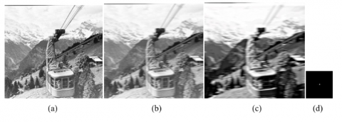
Figure 5. Case of failure of the simple MAP model. The first image (a) Original sharp image (b) Image blurred with a synthetic linear motion blur (c) Deblurred result (d) Estimated PSF
This is because the simple MAP model fails in deblurring the image blurred with a synthetic linear motion blur. This blur adds degradations in the form of shallow edges, medium and narrow peaks very similar to natural images. The MAP model is very effective in deblurring step edges but fails to deblur images with shallow edges, medium and narrow peaks.
A simple MAP model i.e. the MAPh, o will work only on an image dominated by edges. Hence it is not enough for effective utilization for deblurring. The various methods designed to improve the simple MAP model fall short in either deriving accurate convergence to the global optimum or computational implementation. Since convergence of the algorithm is the most important factor for its effectiveness, L0 and L1 norms are theoretically the best regularizers to obtain a better work output. The main problem here is to design an algorithm which can implement them practically. The L2-Relaxed L0 pseudo norm and the L1-Relaxed L0 norm are designed to make the L0 and L1 regularizes computationally implementable. But they are still far from converging to the global optimum. Hence, these criteria required for convergence an algorithm which effectively implements the regularizer to derive the global optimum is a major requirement to improve the existing deblurring methods. Though various methods for image deblurring are designed, they lack in real world, real time implementation and results and commercial success.
The authors acknowledge with thanks JSS Academy of Technical Education, Technical Education Quality Improvement Programme (TEQIP) Cell and Visvesvaraya Technological University (VTU), Belagavi for all the support and encouragement given to them to take up this research work and publication.
|
g |
Blurred and noisy image |
|
|
h |
Blur kernel |
|
|
o |
Deblurred sharp image |
|
|
n |
Additive white Gaussian noise |
|
|
w |
Weights assumed |
|
|
A |
Autonomous blurring |
|
|
I |
Identity Matrix |
|
|
Greek symbols |
|
|
|
a |
Prior in the simple MAP model |
|
|
f |
Prior on o |
|
|
φ |
Prior on h |
|
|
σn |
Standard deviation |
|
|
$\lambda$ |
Data fitting term |
|
|
Subscripts |
|
|
|
h |
Blur kernel |
|
|
o |
Deblurred sharp image |
|
[1] Ribes, A., Schmitt, F. (2008). Linear inverse problems in imaging. IEEE Signal Processing Magazine, 25(4): 84-99. https://doi.org/10.1109/MSP.2008.923099
[2] Gonzalez, R.C., Woods, R.E. (2018). Digital Image Processing. Prentice Hall International Inc., 4th ed.
[3] Hadamard, J. (1923). Lectures on Cauchy’s Problem in Linear Partial Differential Equations. Yale University Press, New Haven.
[4] Šroubek, F., Kamenicky, J., Lu, Y.M. (2016). Decomposition of space-variant blur in image deconvolution. IEEE Signal Processing Letters, 23(3): 346-350. https://doi.org/10.1109/LSP.2016.2519764
[5] Schneider, D., van Ekeris, T., zur Jacobsmuehlen, J., Gross, S. (2013). On benchmarking non-blind deconvolution algorithms: A sample driven comparison of image de-blurring methods for automated visual inspection systems. 2013 IEEE International Instrumentation and Measurement Technology Conference (I2MTC), Minneapolis, MN, pp. 1646-1651. https://doi.org/10.1109/I2MTC.2013.6555693
[6] Kotera, J., Šroubek, F., Milanfar, P. (2013). Blind deconvolution using alternating maximum a posteriori estimation with heavy-tailed priors. Springer International Conference on Computer Analysis of Images and Patterns, pp. 59-66. https://doi.org/10.1007/978-3-642-40246-3_8
[7] Šroubek, F., Milanfar, P. (2011). Robust multichannel blind deconvolution via fast alternating minimization. IEEE Transactions on Image Processing, 21(4): 1687-1700. https://doi.org/10.1109/TIP.2011.2175740
[8] Delbracio, M., Sapiro, G. (2015). Removing camera shake via weighted Fourier burst accumulation. IEEE Transactions on Image Processing, 24(11): 3293-3307. https://doi.org/10.1109/TIP.2015.2442914
[9] Giannakis, G.B., Heath, R.W. (2000). Blind identification of multichannel FIR blurs and perfect image restoration. IEEE Transactions on Image Processing, 9(11): 1877-1896. https://doi.org/10.1109/83.877210
[10] Hosseini, M.S., Plataniot, K.N. (2019). Convolutional deblurring for natural imaging. IEEE Transactions on Image Processing, 29(1): 250-264. https://doi.org/10.1109/TIP.2019.2929865
[11] Faramarzi, E., Rajan, D., Christensen, M.P. (2013). Unified blind method for multi-image super-resolution and single/multi-image blur deconvolution. IEEE Transactions on Image Processing, 22(6): 2101-2114. https://doi.org/10.1109/TIP.2013.2237915
[12] Akay, B., Karaboga, D. (2015). A survey on the applications of artificial bee colony in signal, image, and video processing. Signal, Image and Video Processing, 9(4): 967-990. https://doi.org/10.1007/2Fs11760-015-0758-4
[13] Wang, Y., Yang, J., Yin, W., Zhang, Y. (2008). A new alternating minimization algorithm for total variation image reconstruction. SIAM Journal on Imaging Sciences, 1(3): 248-272. https://doi.org/10.1137/080724265
[14] Anacona-Mosquera, O., Arias-García, J., Muñoz, D.M., Llanos, C.H. (2016). Efficient hardware implementation of the Richardson-Lucy Algorithm for restoring motion-blurred image on reconfigurable digital system. 2016 29th Symposium on Integrated Circuits and Systems Design (SBCCI), Belo Horizonte, pp. 1-6. https://doi.org/10.1109/SBCCI.2016.7724056
[15] Schuler, C.J., Hirsch, M., Harmeling, S., Schölkopf, B. (2016). Learning to deblur. IEEE Transactions on Pattern Analysis and Machine Intelligence, 38(7): 1439-1451. https://doi.org/10.1109/TPAMI.2015.2481418
[16] Xue, F., Blu, T. (2015). A novel SURE-based criterion for parametric PSF estimation. IEEE Transactions on Image Processing, 24(2): 595-607. https://doi.org/10.1109/TIP.2014.2380174
[17] Shah, M.J., Dalal, U. (2017). Single-shot blind uniform motion deblurring with ringing reduction. The Imaging Science Journal, 65(8): 484-499. https://doi.org/10.1080/13682199.2017.1366614
[18] Nagy, J.G., Palmer, K., Perrone, L. (2009). Iterative methods for image deblurring: A Matlab object-oriented approach. Numerical Algorithms, 36(1): 73-93. https://doi.org/10.1023/B:NUMA.0000027762.08431.64
[19] Xiao, L., Gregson, J., Heide, F., Heidrich, W. (2015). Stochastic blind motion deblurring. IEEE Transactions on Image Processing, 24(10): 3071-3085. https://doi.org/10.1109/TIP.2015.2432716
[20] Gregson, J., Heide, F., Hullin, M.B., Rouf, M., Heidrich, W. (2013). Stochastic deconvolution. 2013 IEEE Conference on Computer Vision and Pattern Recognition, Portland, OR, pp. 1043-1050. https://doi.org/10.1109/CVPR.2013.139
[21] Babacan, S.D., Molina, R., Do, M.N., Katsaggelos, A.K. (2012). Bayesian blind deconvolution with general sparse image priors. Springer European Conference on Computer Vision, pp. 341-355. https://doi.org/10.1007/978-3-642-33783-3_25
[22] Tzikas, D.G., Likas, A.C., Galatsanos, N.P. (2009). Variational Bayesian sparse kernel-based blind image deconvolution with student’s-t priors. IEEE transactions on Image Processing, 18(4): 753-764. https://doi.org/10.1109/TIP.2008.2011757
[23] Levin, A., Weiss, Y., Durand, F., Freeman, W.T. (2009). Understanding and evaluating blind deconvolution algorithms. 2009 IEEE Conference on Computer Vision and Pattern Recognition, Miami, FL, pp. 1964-1971. https://doi.org/10.1109/CVPR.2009.5206815
[24] Zuo, W., Ren, D., Zhang, D., Gu, S., Zhang, L. (2016). Learning iteration wise generalized shrinkage-thresholding operators for blind deconvolution. IEEE Transactions on Image Processing, 25(4): 1751-1764. https://doi.org/10.1109/TIP.2016.2531905
[25] Perrone, D., Favaro, P. (2015). A clearer picture of total variation blind deconvolution. IEEE Transactions on Pattern Analysis and Machine Intelligence, 38(6): 1041-1055. https://doi.org/10.1109/TPAMI.2015.2477819
[26] Perrone, D., Favaro, P. (2014). Total variation blind deconvolution: The devil is in the details. Proceedings of the IEEE Conference on Computer Vision and Pattern Recognition, Columbus, OH, pp. 2909-2916. https://doi.org/10.1109/CVPR.2014.372
[27] Padcharoen, A., Kitkuan, D., Kumam, P., Rilwan, J., Kumam, W. (2020). Accelerated alternating minimization algorithm for Poisson noisy image recovery. Inverse Problems in Science and Engineering, 1-26. https://doi.org/10.1080/17415977.2019.1709454
[28] Šroubek, F., Šmídl, V., Kotera, J. (2014). Understanding image priors in blind deconvolution. 2014 IEEE International Conference on Image Processing (ICIP), Paris, pp. 4492-4496. https://doi.org/10.1109/ICIP.2014.7025911
[29] Badri, H., Yahia, H. (2014). Handling noise in image deconvolution with local/non-local priors. 2014 IEEE International Conference on Image Processing (ICIP), Paris, pp. 2644-2648. https://doi.org/10.1109/ICIP.2014.7025535
[30] Ren, W., Tian, J., Tang, Y. (2016). Blind deconvolution with nonlocal similarity and l0 sparsity for noisy image. IEEE Signal Processing Letters, 23(4): 439-443. https://doi.org/10.1109/LSP.2016.2530855
[31] Xu, L., Zheng, S., Jia, J. (2013). Unnatural l0 sparse representation for natural image deblurring. Proceedings of the IEEE Conference on Computer Vision and Pattern Recognition, Portland, OR, pp. 1107-1114. https://doi.org/10.1109/CVPR.2013.147
[32] Zhang, G., Kingsbury, N. (2013). Fast l0-based image deconvolution with variational Bayesian inference and majorization-minimization. 2013 IEEE Global Conference on Signal and Information Processing, Austin, TX, pp. 1081-1084. https://doi.org/10.1109/GlobalSIP.2013.6737081
[33] Xu, L., Jia, J. (2010). Two-phase kernel estimation for robust motion deblurring. European Conference on Computer Vision, pp. 157-170. https://doi.org/10.1007/978-3-642-15549-9_12
[34] Lin, Y., Kandel, Y., Zotta, M., Lifshin, E. (2016). Sem resolution improvement using semi-blind restoration with hybrid l1-l2 regularization. 2016 IEEE Southwest Symposium on Image Analysis and Interpretation (SSIAI), Santa Fe, NM, pp. 33-36. https://doi.org/10.1109/SSIAI.2016.7459168
[35] Huang, Y., Ng, M.K., Wen, Y.W. (2008). A fast total variation minimization method for image restoration. Multiscale Modeling & Simulation, 7(2): 774-795. https://doi.org/10.1137/070703533
[36] Krishnan, D., Tay, T., Fergus, R. (2011). Blind deconvolution using a normalized sparsity measure. IEEE CVPR 2011, Providence, RI, pp. 233-240. https://doi.org/10.1109/CVPR.2011.5995521
[37] Krishnan, D., Fergus, R. (2009). Fast image deconvolution using Hyper-Laplacian priors. Advances in Neural Information Processing Systems, 1033-1041.
[38] Li, Z.M., Zheng, Y., Jing, W.F., Zhao, R.S., Jing, K.L. (2015). Hyper-Laplacian non-blind deblurring model based on regional division. 2015 International Conference on Network and Information Systems for Computers, Wuhan, pp. 223-226. https://doi.org/10.1109/ICNISC.2015.151
[39] Chen, Z., Basarab, A., Kouamé, D. (2015). A simulation study on the choice of regularization parameter in l2-norm ultrasound image restoration. 2015 37th Annual International Conference of the IEEE Engineering in Medicine and Biology Society (EMBC), Milan, pp. 6346-6349. https://doi.org/10.1109/EMBC.2015.7319844
[40] Portilla, J., Tristán-Vega, A., Selesnick, I.W. (2015). Efficient and robust image restoration using multiple-feature l2-relaxed sparse analysis priors. IEEE Transactions on Image Processing, 24(12): 5046-5059. https://doi.org/10.1109/TIP.2015.2478405
[41] Perona, P. Malik, J. (1990). Scale-space and edge detection using anisotropic diffusion. IEEE Transactions on Pattern Analysis and Machine Intelligence, 12(7): 629-639. https://doi.org/10.1109/34.56205
[42] You, Y.L., Kaveh, M. (1999). Blind image restoration by anisotropic regularization. IEEE Transactions on Image Processing, 8(3): 396-407. https://doi.org/10.1109/83.748894
[43] Chan, T.F., Wong, C.K. (1998). Total variation blind deconvolution. IEEE Transactions on Image Processing, 7(3): 370-375. https://doi.org/10.1109/83.661187
[44] Liu, H.J., Gu, M., Meng, Q.H., Lu, W.S. (2016). Fast weighted total variation regularization algorithm for blur identification and image restoration. IEEE Access, 4: 6792-6801. https://doi.org/10.1109/ACCESS.2016.2516949
[45] Chen, K. (2013). Introduction to variational image-processing models and applications. International Journal of Computer Mathematics, 90(1): 1-8. https://doi.org/10.1080/00207160.2012.757073
[46] Shrivakshan, G., Chandrasekar, C. (2012). A comparison of various edge detection techniques used in image processing. International Journal of Computer Science Issues (IJCSI), 9(5): 269-281. https://doi.org/10.13140/RG.2.1.5036.7123
[47] McGaffin, M.G., Fessler, J.A. (2015). Edge-preserving image denoising via group coordinate descent on the GPU. IEEE Transactions on Image Processing, 24(4): 1273-1281. https://doi.org/10.1109/TIP.2015.2400813
[48] Cho, S., Lee, S. (2009). Fast motion deblurring. ACM Transactions on Graphics (TOG), 28(5): 145-156. https://doi.org/10.1145/1618452.1618491
[49] Hanif, M., Seghouane, A.K. (2014). Blind image deblurring using non negative sparse approximation. 2014 IEEE International Conference on Image Processing (ICIP), Paris, pp. 4042-4046. https://doi.org/10.1109/ICIP.2014.7025821
[50] Shearer, P., Gilbert, A.C., Hero, A.O. (2013) Correcting camera shake by incremental sparse approximation. 2013 IEEE International Conference on Image Processing, Melbourne, VIC, pp. 572-576. https://doi.org/10.1109/ICIP.2013.6738118
[51] Michaeli, T., Irani, M. (2014). Blind deblurring using internal patch recurrence. Springer European Conference on Computer Vision, pp. 783-798. https://doi.org/10.1007/978-3-319-10578-9_51
[52] Zontak, M., Irani, M. (2011). Internal statistics of a single natural image. IEEE CVPR 2011, Providence, RI, pp. 977-984. https://doi.org/10.1109/CVPR.2011.5995401
[53] Mohd Shapri, A.H., Abdullah, M.Z. (2017). Accurate retrieval of region of interest for estimating point spread function and image deblurring. The Imaging Science Journal, 65(6): 327-348. https://doi.org/10.1080/13682199.2017.1341457
[54] Kotera, J., Zitová, B., Šroubek, F. (2015). PSF accuracy measure fore valuation of blur estimation algorithms. in 2015 IEEE International Conference on Image Processing (ICIP), Quebec City, QC, pp. 2080-2084. https://doi.org/10.1109/ICIP.2015.7351167