Huadong Wang
© 2020 IIETA. This article is published by IIETA and is licensed under the CC BY 4.0 license (http://creativecommons.org/licenses/by/4.0/).
OPEN ACCESS
The bit error induced by the chaotic noise is a serious problem among weak harmonic signal detection methods for wireless network environment. To solve the problem, this paper puts forward a weak harmonic signal detection method for network environment with chaotic noise. Firstly, the real-time transmission signal was collected from the wireless network, and the noise signal was extracted and suppressed in the light of the chaotic features of the signal. In this way, the detection accuracy of weak harmonic signal will not be affected by the noise signal. Then, the detection amplitude and frequency were determined according to the effective values of harmonic components and harmonic frequency, facilitating the detection of weak harmonic signal. Experimental results show that our method outputted a lower bit error rate (BER) than existing methods in weak harmonic signal detection, and outperformed the contrastive methods in reliability and performance.
chaotic noise, wireless network, weak signal, harmonic signals, signal detection, bit error rate (BER)
Wireless telecommunication network, as the combination of wireless network and telecommunication network, supports information exchange and sharing. This network is generally applied in the remote control and transmission of electromagnetic waves, showing a great significance in life and work. The safe and stable operation of the wireless network is threatened by the harmonics and inter-harmonics. Originating from the massive use of nonlinear loads, the harmonics in wireless network cause the failure of various network equipment and disrupt the normal data communication [1]. For the stability of wireless network, it is necessary to suppress or eliminate harmonics in the network. As a result, a harmonic signal detection method should be designed to answer two questions: Whether the wireless network contains harmonic signal? Where is the location of the harmonic signal?
The harmonic signal, generally weak in the wireless network, cannot be detected accurately by a low-precision method. The difficulty in detecting weak harmonic signal is amplified by the chaotic noise produced in the operation of the wireless network. In the wireless network, the chaotic noise exists as an unstable noise factor with unobvious rules. Chaos is an irregular and unstable state of motion that generally exists in nonlinear systems, regardless of the system scale. Unique to deterministic nonlinear dynamic systems, chaotic motions are featured by internal stochasticity, global stability, local instability, sensitive dependence, ergodicity, orbital instability, to name but a few. In the presence of chaotic noise, the key to the detection of weak signal is to judge whether all or part of the signal are abnormal [2].
At present, the weak signal in the wireless network is mainly detected based on sparse decomposition (SD), wavelet entropy (WE), or the fluctuation of frequency amplitude. However, the existing methods cannot accurately capture weak harmonic signal in actual application environment, which is severely disturbed by chaotic background noise. To solve the problem, the features of chaotic noise and target signal should be further analyzed, and used to design a signal detection method with better accuracy and applicability. Focusing on the chaotic noise environment, this paper optimizes the traditional signal detection method, and puts forward an effective way to detect weak harmonic signal in the wireless network.
To detect weak signal, it is necessary to examine the law of noise and the features of signal, and then extract and measure the weak signal features from the chaotic noise background, using a series of signal processing methods [3]. Before signal detection, the chaotic signal, network signal, and noise signal should be separated from the collected equal interval signal. Then, the noise data should be removed from the signal to facilitate the detection of the target signals. Finally, the weak harmonic signal can be detected accurately based on the chaotic oscillator and periodic features of the chaotic signal.
2.1 Real-time signal acquisition and processing
To detect weak harmonic signal in the wireless network, the first step is to acquire the signal transmitted in the network at different intervals. The input signal of the wireless network can be described as:
$s(k)=A \sin \left(2 \pi f k+\varphi_{0}\right)$ (1)
where, A, f, and φ0 are the amplitude, frequency, and original phase of the input signal, respectively [4]. Then, the sampling interval of wireless network signal can be calculated by:
$T_{N}=\frac{1+N}{N f}$ (2)
where, N is the conversion coefficient of wireless network signal.
Let 1/Ts be the acquisition rate of wireless network signal. Then, the collected weak signal can be expressed as a time sequence:
$s(y)=A \sin \left(2 \pi f y\left(\frac{1}{N f}+\frac{1}{f}\right)+\varphi_{0}\right)$ (3)
where, y is the number of signal samples. Combining formulas (1) and (3), the collected weak signal can be depicted as:
$\left\{\begin{array}{l}T=\frac{N+1}{f} \\ f_{\varphi}=\frac{f}{N+1} \\ s_{\varphi}=A \sin \left(2 \pi f_{\varphi} y+\varphi_{0}\right)\end{array}\right.$ (4)
where, fφ is the frequency of the collected weak signal. Then, the initial modal components of the collected signal can be separated by:
$s_{\rho}=\sum_{j=1}^{n} c_{j}(t)+r_{n}(t)$ (5)
where, cj(t) is the j-th modal component separated from the collected signal; rn(t) is the residual signal after the n-th separation [5].
2.2 Separation of chaotic noise signal
The collected weak signal contains some chaotic noise signal, for the wireless network is disturbed by chaotic noise. The chaotic noise signal will dampen the detection accuracy of weak harmonic signal [6]. Therefore, the chaotic noise signal should be separated from the collected signal, and eliminated based on the chaotic features.
2.2.1 Feature analysis of chaotic oscillator
Suppose f(x) features continuous self-mapping in the closed interval [a, b]. Then, a noise is a chaotic noise, if it satisfies the following two conditions: (1) Periodic points exist in f(x); (2) There exists an uncountable subset $S \in I$ that satisfies:
$\left\{\begin{array}{l}\forall x, y \in S \& x \neq y, \lim _{n \rightarrow \infty} \sup \left|f^{n}(x)-f^{n}(y)\right|>0 \\ \forall x, y \in S, \liminf _{n \rightarrow \infty}\left|f^{n}(x)-f^{n}(y)\right|=0 \\ \forall x \in S, \liminf _{n \rightarrow \infty}\left|f^{n}(x)-f^{n}(y)\right|=0\end{array}\right.$ (6)
where, sup(⋅) and inf(⋅) are the upper and lower bounds, respectively; fn(⋅) is the n-th iteration of f. The noise content of the collected signal can be measured by signal-to-noise ratio (SNR) and noise level. The modal components of the collected signal can be expressed as a time sequence:
$s(t)=x(t)+n(t)$ (7)
where, x(t) and n(t) are pure time sequence and additive noise, respectively. Then, the noise level of a modal component can be computed by:
$N_{l}=\sqrt{\frac{\sigma(n(t))}{\sigma(x(t))}}$ (8)
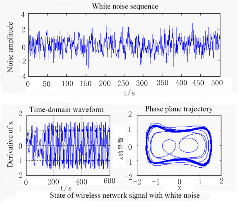
where, σ(⋅) is the variance of the time sequence. The trajectory of chaotic signal varies with the noise disturbances [7]. Taking white noise for example, the features of the wireless network signal with white noise are compared in Figure 1 below.
Figure 1. The features of the wireless network signals with white noise
As shown in Figure 1, the chaotic oscillator is immune to noise: the changing noise intensity merely affected the trajectory in the phase diagram, and had little to do with the state of the chaotic signal.
2.2.2 Feature extraction of chaotic noise
Based on the results of feature analysis and the properties of chaotic oscillator, the features of chaotic noise can be extracted [8], including Lyapunov exponent, correlation dimension, and Kolmogorov entropy. Among them, the correlation dimension can be calculated by:
$\left\{\begin{array}{l}\dot{x}=\eta(y-x) \times N_{l} \\ y=-x+7 x-y \times N_{i} \\ \dot{z}=x y-b z \times N_{l}\end{array}\right.$ (9)
where, η, b and r are three constant terms. Then, x, y and z were initialized as 1, 0, and 0.1. Substituting the chaotic noise points in the time sequence of chaotic signal into formula (9), the correlation dimension of chaotic noise can be obtained. The values of other features can be obtained in a similar manner.
2.2.3 Suppression of noise signal
The extracted features of chaotic noise were utilized to determine the minimum embedding dimension of the time sequence for wireless network signal, and to differentiate between deterministic and stochastic time sequences. In this way, the chaotic noise can be separated from the collected signal. In addition, the noise in the wireless network signal was suppressed by the noise cancellation device in Figure 2, where the inputs are the collected signal and the predicted signal after noise suppression; eφ(n) is the error sequence in noise cancellation.
Figure 2. Structure of the noise cancellation device
2.3 Calculation of effective values of harmonic components
Let g(t) and g(n) be the weak signal of the wireless network after noise suppression and its corresponding digital signal, respectively. Then, the following can be derived by weighting the wavelet basis function:
$\int x(t)^{2}=\sum_{i=0}^{\eta} \sum_{k=0}^{2^{j}-1}\left(d_{j}^{i}(k)-g(t)\right)^{2} \times(\dot{x}+\dot{y}+\dot{z})$ (10)
where, dij(k) is the coefficient of the scale function. Then, the root mean square (RMS) of the wireless network signal can be expressed as:
$X_{\text {тт5}}=\sqrt{\sum_{i=0}^{2^{j}-1}\left(V_{j}^{i}\right)^{2}}$ (11)
where, Vij is the effective value of harmonic components in different frequency bands:
$V_{j}^{i}=\sqrt{\frac{1}{2^{N}} \sum_{k=0}^{2^{N-j-1}}\left(d_{j}^{i}(k)\right)^{2}}$ (12)
Then, the effective value of harmonic components in the wireless network signal can be obtained by reverse deduction.
2.4 Solution of harmonic frequency
Based on the effective values of harmonic components in the wireless network signal, the harmonic matrix was constructed, and the eigenvalue of covariance matrix R was computed. Then, the likelihood function can be solved by substituting the eigenvalue into the following formula:
$\Lambda(n)=V_{j}^{i} \frac{1}{M-n} \times \frac{\sum_{i=n+1}^{M} \lambda_{i}}{\left(\prod_{i=n+1}^{M} \lambda_{i}\right)^{\frac{1}{M-n}}}$ (13)
where, M is the number of array elements of the signal; n is the number of harmonic components; λi is the eigenvalue of covariance matrix R of signal X. Next, the function expressed by formula (13) was represented by a curve. The number of inflection points on the curve is the number of harmonic signals in the wireless network signal [9]. Then, the eigenvalues of covariance matrices were sorted in descending order, creating the eigenvector matrix. On this basis, the frequency of each harmonic component can be estimated by:
$f_{k}=\frac{\operatorname{angle}\left(\lambda_{i}\right)}{2 \pi T_{s}}$ (14)
where, λk is the composite eigenvalue of the eigenvector matrix.
2.5 Determination of the amplitude and frequency for weak signal detection
Under the background of chaotic noise, the frequency of weak periodic signal can be expressed as:
$r(t)=\frac{k(t)+m(t)}{f_{k}}$ (15)
where, k(t) is the weak sine harmonic signal of the wireless network; m(t) is the white noise signal with an SNR<-20dB. To determine the detection frequency, the frequency of weak sine harmonic signal should be estimated first [10]. Considering the structural variation in chaotic coefficient, the SNR curve with synchronization error can be obtained (Figure 3).
Figure 3. The SNR-frequency curve
As shown in Figure 3, the SNR exhibited a decline with the growing frequency of the input signal [11-15]. Considering the synchronization error of the chaotic noise background, the detection threshold for weak harmonic signal was set to -15dB. Under the current parameters, the effective interval of detection frequency was obtained as [0Hz, 200Hz].
The critical threshold for chaotic signal and detection amplitude of sine signal were derived from the effective values of harmonic components. To obtain an accurate critical threshold, the position of the threshold was approximated based on the amplitude bifurcation [16-20].
Let P1 and P2 correspond to the chaotic state and periodic state of the noise signal, respectively. The threshold could fall on the halfway between P1 and P2, i.e. x= $\frac{P_{1}+P_{2}}{2}$ . Since $\frac{P_{1}+P_{2}}{2}$ and $\frac{P_{1}+P_{2}}{2}$ + 0.1 both correspond to the chaotic state and $\frac{P_{1}+P_{2}}{2}$ +0.2 corresponds to the periodic state, the interval of f can be determined as $\left[\frac{P_{1}+P_{2}}{2}+0.1, \frac{P_{1}+P_{2}}{2}+0.2\right]$ . In this interval, the compensation was increased with a step of 0.001, such as to find the transition point from the chaotic state to the periodic state. This point was taken as the critical threshold for signal detection.
At the critical threshold, the target wireless network signal was mixed with noise, and used to perturb the chaotic oscillator. By observing the variation of phase trajectory, all the sine signals of the weak harmonics were identified from the mixed signal. After that, the amplitude position was adjusted again and the noisy signal was controlled at the critical threshold of chaotic state, creating a new threshold. Therefore, the sine signal amplitude of the input mixed signal can be computed by:
$A=r(t) \times\left(\gamma_{1}-\gamma_{2}\right)$ (16)
where, γ1 and γ2 are the initial critical threshold and the new threshold, respectively.
2.6 Detection of weak harmonic signal
According to the effective values of harmonic components, detection amplitude and detection frequency, the collected signal that contains chaotic noise and the determined detection signal were inputted at the same time. Then, we have:
$\left\{\begin{array}{l}\ddot{x}+\alpha_{1}\left[\left(x^{2}+y^{2}+z^{2}\right)-1\right] \dot{x}+\beta_{1} x= \\ f_{\mathrm{e}} \cos (\omega t+\theta)+a \cos (\omega t+\theta)+n(t) \\ \dot{y}+\alpha_{2}\left[\left(x^{2}+y^{2}+z^{2}\right)-1\right] \dot{y}+\beta_{2} y= \\ f_{\mathrm{e}} \cos (\omega t+\theta)+a \cos (\omega t+\theta)+n(t) \\ \ddot{z}+\alpha_{3}\left[\left(x^{2}+y^{2}+z^{2}\right)-1\right] \dot{z}+\beta_{3} z= \\ f_{\mathrm{e}} \cos (\omega t+\theta)+a \cos (\omega t+\theta)+n(t)\end{array}\right.$ (17)
where, acos(ωt+θ) is the weak harmonic signal of the wireless network; a is the amplitude of the weak harmonic signal. If the weak sine signal and the chaotic noise signal are of the same period, frequency, and phase, the chaotic signal will be sensitive to the weak sine signal, while immune to the noise. Hence, the phase trajectory of the resulting chaotic signal will quickly change from chaotic state to periodic state. Once the change takes place, the weak harmonic signal can be detected successfully [21, 22].
If the chaotic noise in the background is uniform, the detection amplitude and frequency for nonuniform chaotic noise background can be adjusted before detecting the weak harmonic signal in the wireless network. In addition, the transient signal of the weak harmonic signal can be described by:
$\left\{\begin{array}{l}H_{0}: x(n)=c(n) \\ H_{1}: x(n)=c(n)+s(n)\end{array}\right.$ (18)
where, H0 and H1 are two states of wireless network. The two states have different transient signals. Therefore, the harmonic signals detected at the two states must be different. Similarly, the periodic signal of weak harmonic signal can be detected, according to the chaotic moving features of the harmonic signal in the wireless network.
3.1 Experimental purpose
Our experiments attempt to verify the effects of the proposed method in detecting actual weak harmonic signal of the wireless network, demonstrate the superiority of our method over existing methods in detection accuracy, and indirectly prove the application value of our method in actual wireless networks.
3.2 Experimental environment
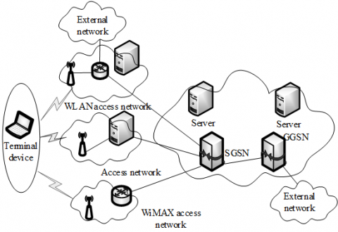
There are roughly two parts of the experimental environment: the implementation environment of our method, and the operation environment of our method. The former must have wireless network signals with harmonic components. The topology of the wireless network constructed for experiments is displayed in Figure 4.
Figure 4. Topology of wireless network
According to the topology in Figure 4, the servers and terminal devices were installed in the experimental environment, and wirelessly interconnected via a router. To collect different wireless network signals, the terminal devices in the environment are of different models and forms.
The implementation environment is responsible for converting our method into a code that can be directly read and run by computer, using a lossless compression and encoding method, and import the code into any terminal device in the wireless network. The device inputted with the code was defined as the main testing computer.
In addition to the encoding program, the designed core cannot function normally without a suitable hardware environment. Therefore, the internal wiring of the main testing computer was modified into the weak harmonic signal detection circuit (Figure 5).
Figure 5. Weak harmonic signal detection circuit
Our method aims to improve the detection accuracy of weak harmonic signal in wireless network under different noise disturbances. Hence, Gaussian white noises of varied intensities were introduced to the basic experimental environment. All experimental data were processed on MATLAB.
3.2 Performance metric
The signal detection performance was measured by the BERs under different SNRs. The BER is the ratio of the output signal to the preset signal. During the experiments, the detection results were recorded, and divided by the present data to obtain the BERs of our method.
3.3 Input signal
Under the experimental environment, the signal output of the wireless network was controlled, and the parameters of the input signal were configured as in Table 1, where A is the signal amplitude; B is a random parameter; φ is the phase value.
Table 1. Parameters of input signal
|
|
A |
B |
φ |
|
S1 |
3×10⁻⁴ |
1×10⁻³ |
0 |
|
S2 |
3×10⁻¹ |
1 |
0 |
|
S3 |
3×10⁻¹ |
0 |
0 |
|
S4 |
3×10⁻⁴ |
6×10⁻² |
0 |
|
S5 |
3×10⁻⁴ |
8×10⁻² |
0 |
3.4 Experimental procedure
The prepared initial signals were imported to the main testing computer, and processed by our method to obtain the detection results. The SD-based method and WE-based method were selected as the contrastive methods. The SD-based method searches for the signals with the same eigenvalues as the target harmonic signal, extracts all these signals, and output them as the detection result. Drawing on the result of the SD-based method, the WE-based method detects weak harmonic signal in the light of its coupling features. The two contrastive methods were introduced to the experimental environment in the same manner as our method.
3.5 Comparison of detection results
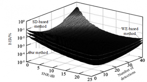
The BERs of our method, SD-based method and WE-based method were computed based on their detection results, and compared in Figure 7 below.
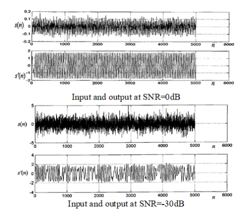
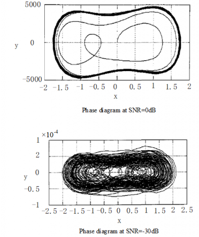
(a) Waveform
(b) Phase diagram
Figure 6. Initial waveform and phase diagram of signal S1
Figure 7. The BERs of the three methods
As shown in Figure 7, with the growing number of detections and SNR, the BERs of all three methods were declining. When the SNR was the same, our method achieved the lowest BER, reflecting its superiority than the two contrastive methods in weak harmonic signal detection. The superiority comes from the extraction and suppression of noise signal as per the chaotic features of signal. The noise suppression mitigates the effects of noise signal on the detection accuracy of weak harmonic signal, making our method more accurate and reliable.
To sum up, our method can effectively detect the weak harmonic signals in the wireless network under different conditions. Compared with the existing methods, our approach has significant advantages in terms of BER. The proposed method enjoys great application value, and provides a guarantee for the security of wireless network.
The high BER is a common problem among the existing detection methods for weak harmonic signal. To overcome the problem, this paper proposes a novel method to detect weak harmonic signal in wireless network under chaotic noise. The theoretical basis of our method lies in the discrimination between chaos and noise. Drawing on the features of harmonic signal and chaos under noise, the harmonic signal was detected in the wireless network, and used to adjust the operation parameters of the network in time, making the network operation safe and stable. Experimental results show that our method outputted reliable results at different SNRs, and achieved a much lower BER than the existing methods. Of course, the experimental results have certain limitations, because the input signal was only disturbed by Gaussian white noise. The future research will improve and verify the effect of our method in the presence of colored noise and other noises.
This work is supported by the School-based Program of Zhoukou Normal University (Grant No.: ZKNUB2201803).
[1] Zhou, J., Chen, J., Shan, Z. (2017). Spatial signature analysis of submarine magnetic anomaly at low altitude. IEEE Transactions on Magnetics, 53(12): 1-7. https://doi.org/10.1109/TMAG.2017.2735940
[2] Sheinker, A., Salomonski, N., Ginzburg, B., Frumkis, L., Kaplan, B.Z. (2008). Magnetic anomaly detection using entropy filter. Measurement Science and Technology, 19(4): 045205. https://doi.org/10.1088/0957-0233/19/4/045205
[3] Kakarala, R., Ogunbona, P.O. (2001). Signal analysis using a multiresolution form of the singular value decomposition. IEEE Transactions on Image Processing, 10(5): 724-735. https://doi.org/10.1109/83.918566
[4] Lu, S., He, Q., Wang, J. (2019). A review of stochastic resonance in rotating machine fault detection. Mechanical Systems and Signal Processing, 116: 230-260. https://doi.org/10.1016/j.ymssp.2018.06.032
[5] Benzi, R., Sutera, A., Vulpiani, A. (1981). The mechanism of stochastic resonance. Journal of Physics A: Mathematical and General, 14(11): L453. https://doi.org/10.1088/0305-4470/14/11/006
[6] Wan, C., Pan, M., Zhang, Q., Wu, F., Pan, L., Sun, X. (2018). Magnetic anomaly detection based on stochastic resonance. Sensors and Actuators A: Physical, 278: 11-17. https://doi.org/10.1016/j.sna.2018.05.009
[7] Wang, C., Huang, N., Bai, Y., Zhang, S. (2018). A method of network topology optimization design considering application process characteristic. Modern Physics Letters B, 32(7): 1850091. https://doi.org/10.1142/S0217984918500914
[8] Diamant, R., Francescon, R., Zorzi, M. (2017). Topology-efficient discovery: A topology discovery algorithm for underwater acoustic networks. IEEE Journal of Oceanic Engineering, 43(4): 1200-1214. https://doi.org/10.1109/JOE.2017.2716238
[9] Cavraro, G., Arghandeh, R. (2017). Power distribution network topology detection with time-series signature verification method. IEEE Transactions on Power Systems, 33(4): 3500-3509. https://doi.org/10.1109/TPWRS.2017.2779129
[10] Lee, K., Wu, Y., Bresler, Y. (2017). Near-optimal compressed sensing of a class of sparse low-rank matrices via sparse power factorization. IEEE Transactions on Information Theory, 64(3): 1666-1698. https://doi.org/10.1109/TIT.2017.2784479
[11] Han, X., Shen, Z., Wang, W. X., Di, Z. (2015). Robust reconstruction of complex networks from sparse data. Physical Review Letters, 114(2): 028701. https://doi.org/10.1103/PhysRevLett.114.028701
[12] Parsegov, S.E., Proskurnikov, A.V., Tempo, R., Friedkin, N.E. (2016). Novel multidimensional models of opinion dynamics in social networks. IEEE Transactions on Automatic Control, 62(5): 2270-2285. https://doi.org/10.1109/TAC.2016.2613905
[13] Corsini, G., Mossa, A., Verrazzani, L. (1996). Signal-to-noise ratio and autocorrelation function of the image intensity in coherent systems. Sub-Rayleigh and super-Rayleigh conditions. IEEE Transactions on Image Processing, 5(1), 132-141. https://doi.org/10.1109/83.481677
[14] Yatsenko, V., Kolesnik, Y., Titarenko, T. (1994). Identification of the non-Gaussian chaotic dynamics of the radioemission back scattering processes. IFAC Proceedings Volumes, 27(8): 277-281. https://doi.org/10.1016/S1474-6670(17)47728-7
[15] Mukherjee, S., Osuna, E., Girosi, F. (1997). Nonlinear prediction of chaotic time series using support vector machines. In Neural Networks for Signal Processing VII. Proceedings of the 1997 IEEE Signal Processing Society Workshop, pp. 511-520. https://doi.org/10.1109/NNSP.1997.622433
[16] Leung, H., Hennessey, G., Drosopoulos, A. (2000). Signal detection using the radial basis function coupled map lattice. IEEE Transactions on Neural Networks, 11(5): 1133-1151. https://doi.org/10.1109/72.870045
[17] Sakai, K., Noguchi, Y., Asada, S.I. (2008). Detecting chaos in a citrus orchard: Reconstruction of nonlinear dynamics from very short ecological time series. Chaos, Solitons & Fractals, 38(5): 1274-1282. https://doi.org/10.1016/j.chaos.2007.01.144
[18] Zadeh, A.E. (2010). Automatic recognition of radio signals using a hybrid intelligent technique. Expert Systems with Applications, 37(8): 5803-5812. https://doi.org/10.1016/j.eswa.2010.02.027
[19] Xing, H.Y., Jin, T.L. (2010). Weak signal estimation in chaotic clutter using wavelet analysis and symmetric LS-SVM regression. Acta Physica Sinica, 59(1): 140-146. https://doi.org/10.7498/aps.59.140
[20] Pan, G., Li, K., Ouyang, A., Li, K. (2016). Hybrid immune algorithm based on greedy algorithm and delete-cross operator for solving TSP. Soft Computing, 20(2): 555-566. https://doi.org/10.1007/s00500-014-1522-3
[21] Kugiumtzis, D. (1996). State space reconstruction parameters in the analysis of chaotic time series—the role of the time window length. Physica D: Nonlinear Phenomena, 95(1): 13-28. https://doi.org/10.1016/0167-2789(96)00054-1
[22] Chang, C.C., Lin, C.J. (2011). LIBSVM: A library for support vector machines. ACM Transactions on Intelligent Systems and Technology (TIST), 2(3): 1-27. https://doi.org/10.1145/1961189.1961199