Hao Wu* | Xiaoyan Sun | Yanan Liu | Dagang Wang | Bing Wei
© 2020 IIETA. This article is published by IIETA and is licensed under the CC BY 4.0 license (http://creativecommons.org/licenses/by/4.0/).
OPEN ACCESS
In vehicle image segmentation, the traditional graph cut algorithm often have errors, when the original image contains shadows or complex background. To overcome the errors, this paper introduces the shape prior to graph cut algorithm. Our algorithm firstly maps the vehicle image to a weighted undirected graph, and obtains the regional energy and boundary energy functions. Then, the shape prior was added to constrain the image segmentation, and create a new energy function. The star convex was selected as the shape prior, and manually marked. Experimental results show that our algorithm segmented complex background vehicle images, shadowed vehicle images, and incomplete vehicle images more effectively than Otsu’s method and graph cut algorithm. The details of vehicles were preserved and extracted efficiently by our algorithm. The research results provide new insights into vehicle image segmentation.
shape prior, graph cut, image segmentation, vehicle images
Image segmentation is the process of segmenting the region of interest (ROI) in a complete image. It is the prerequisite for advanced image processing techniques like image analysis, object recognition, and object tracking. Therefore, image segmentation is a research hotspot of image processing [1].
Over the years, many image segmentation algorithms have emerged, taking basis on threshold, edge detection, deep learning, or graph theory [2]. Boykov and Jolly [3] proposed the graph cut algorithm, an image segmentation algorithm based on graph theory, which has relatively high segmentation accuracy. On this basis, Rother et al. [4] developed the GrabCut algorithm. An [5] introduced the texture features of the object to the energy function of graph cut algorithm. Hou [6] combined the graph cut algorithm with the level set technique. Through deep learning, Pi [7] selected seed points of object and background pixels.
In recent years, many scholars have attempted to fuse graph cut and shape prior model. The fused results include parameter-adaptive shape prior constraint algorithm based on kernel principal component analysis (KPCA), adaptive shape prior model [8], and graph cut and nonlinear statistical shape prior algorithm [9]. For the effectiveness of image segmentation, some scholars included image features like color, grayscale, and texture into the algorithm design [10].
Vehicle image segmentation is critical to vehicle image analysis and vehicle tracking. The segmentation results directly affect vehicle detection and other subsequent processing [11]. The research of vehicle image segmentation has a great application value, laying a solid basis for intelligent transport [12].
There are two common mistakes in vehicle image segmentation: the complex background, lanes, buildings and shadows are often incorrectly recognized as objects, while the boundaries that divide the vehicle body from windows and wheels are often mistook as non-objects [13].
Considering the features of vehicle images, this paper designs a vehicle image segmentation algorithm that fuses vehicle shape features and graph cut algorithm. The vehicle shape features prevent the segmentation from the interference of shadows and complex background, while the graph cut algorithm effectively segments the boundaries of windows and wheels. The proposed algorithm is simple to design and high in accuracy.
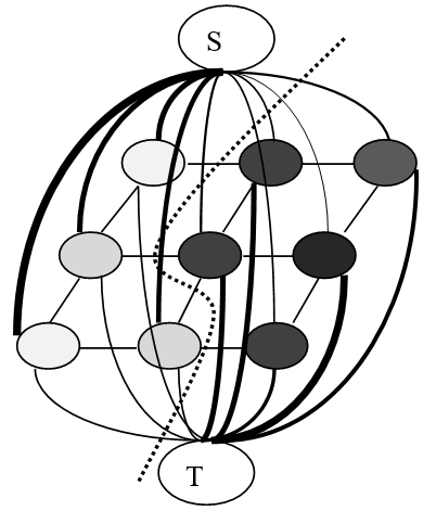
Graph cut algorithm is an image segmentation algorithm based on graph theory. The basic idea of the algorithm was explained with a 3×3 digital image (Figure 1) and its weighted undirected graph (Figure 2). In Figure 2, the darkness of each pixel represents its grayscale; S is the source node of object pixels; T is the sink node of background pixels. S is directly connected to all the other nodes except T, and T is directly connected to all the other nodes except S [14].
Figure 1. The 3×3 digital image
Figure 2. The S-T weighted undirected graph
Graph cut algorithm aims to segment the digital image into a binary image: all object pixels are recorded as 1, and all background pixels as 0. In essence, an energy function is designed based on edge weights, and minimized to segment the image. The energy function of graph cut algorithm is designed as follows:
Let L={l1,l2,l3,…,ln} be the set of pixels in the digital image. The energy function can be defined as:
$E(L)=\lambda R(L)+B(L)$ (1)
where, E(L) is the energy of graph cut algorithm; R(L) is the regional energy corresponding to the weights of t-links; B(L) is the boundary energy corresponding to the weights of n-links. The above formula integrates the regional and boundary features of the digital image. The value of R(L) can be computed by:
$R(L)=\sum\limits_{{{l}_{i}}\in L}{{{R}_{{{l}_{i}}}}({{l}_{i}})}$ (2)
where, liis a pixel in the digital image, and an element of set L. The penalty of whether pixel libelongs to object or background can be expressed as:
${{R}_{{{l}_{i}}}}('obj')=-{{\log }_{2}}\left( \left. \frac{su{{m}_{{{l}_{i}}}}}{su{{m}_{obj}}} \right) \right.$ (3)
${{R}_{{{l}_{i}}}}('bkg')=-{{\log }_{2}}\left( \left. \frac{su{{m}_{{{l}_{i}}}}}{su{{m}_{bkg}}} \right) \right.$ (4)
where, sumli is the number of pixels that satisfy the required pixel values; sumbkg and sumobj are the number of background pixels and object pixels tagged by the user, respectively.
If pixel li belongs to the object, the probability of the pixel belonging to object is greater than the probability of the pixel belonging to background, i.e. Rli(0)>Rli(1). Formulas (3) and (4) ensure that pixel li is given a tag (i.e. object or background) with the higher probability, which minimizes the energy. If all pixels are classified correctly, then the regional energy will minimize [16].
The boundary energy mainly considers the boundary attribute of the object:
$B(L)=\sum\limits_{\{{{l}_{i}},{{l}_{j}}\}}{{{B}_{\{{{l}_{i}},{{l}_{j}}\}}}\delta ({{l}_{i}},{{l}_{j}})}$ (5)
$\delta ({{l}_{i}},{{l}_{j}})=\left\{ \begin{matrix} 0\begin{matrix}, & {{l}_{i}}={{l}_{j}} \\\end{matrix} \\ 1\begin{matrix}, & {{l}_{i}}\ne {{l}_{j}} \\\end{matrix} \\\end{matrix} \right.$ (6)
where,
${{B}_{\{{{l}_{i}},{{l}_{j}}\}}}=\exp \left( \frac{{{({{l}_{i}}-{{l}_{j}})}^{2}}}{2{{\delta }^{2}}} \right)$ (7)
where, li and lj are two adjacent pixels. If the two pixels have similar values, there is a high probability that they belong to the same class. In this case, B{li ,lj }will have a large value. If the two pixels have very different values, then they fall on the edges of the object and the background, i.e. the dividing line between object and background. In this case, B{li ,lj }will be close to zero.
The best segmentation effect can be achieved by minimizing the value of the energy function, i.e. performing the minimum cut [17]. Therefore, the key of graph cut algorithm is to find the optimal solution of the energy function [18].
This paper introduces shape prior information, i.e. the object perceived as the ROI in advance, into image processing. Take vehicle image segmentation for example. The shape prior information refers to the vehicle in the image. Shape, as a visual feature of the image, can greatly enhance the accuracy of image segmentation.
3.1 Shape constraint
The shape prior constraint reflects the intuitive information of the digital image. Many shape prior image segmentation algorithms have been developed. But many algorithms are not highly universal, for shapes like convex and ellipse only applies to a narrow range of objects. The shape prior for vehicle image segmentation must be universal, due to the complexity of vehicle images. The star convex was selected thanks to its applicability to various complex objects [19].
The star convex set is a fusion of mathematical and geometric knowledge. Vekslerwas the first to applythe set to image segmentation [20]. In this paper, the vehicle image to be segmented is denoted as Ω. The shape of the star convex is illustrated in Figure 3, where Ωi is a constraint set about center O; C is the boundary of the object.
Figure 3. The shape of the star convex
Ωi is also the object region of the vehicle image. If the straight line linking up center O and curve C always falls into the object region, then the object region can be regarded as the convex prior about center O.
For the binary segmentation image (object pixels: 1; background pixels: 0), the constraint cost of the star convex prior can be defined by the straight line passing through center O and lj:
For any
${{l}_{i}}\in {{\Gamma }_{o,{{l}_{j}}}},f(C\left| o \right.)=\left\{ \begin{matrix} \infty \begin{matrix}, if & C\in {{\Omega }_{i}} \\\end{matrix} \\ 0,\begin{matrix} if & C\notin {{\Omega }_{i}} \\\end{matrix} \\\end{matrix} \right.$ (8)
${{F}^{*}}\left( C\left| o \right. \right)=\oint{_{{{\Gamma }_{o,{{l}_{j}}}}}}f\left( C\left| o \right. \right)dxdy$ (9)
For the digital vehicle image, the entire vehicle image Ω is a set of discrete data; O, li, and ljare the pixels in the image [15].
The star convex constraint is very flexible for vehicle objects. A single vehicle can have a starconvex constraint about the center, so does an incomplete vehicle. Figure 4 shows the starconvex shapes of actual vehicles, including incomplete vehicles.
Figure 4. The star convex shapes of vehicles
To effectively segment the vehicle, this paper introduces the shape constraint of star convex prior to the energy function of graph cut algorithm, turning the energy function into:
$E=\lambda \sum\limits_{{{l}_{i}}\in L}{{{R}_{{{l}_{i}}}}\left( {{l}_{i}} \right)+\sum\limits_{\left\{ {{l}_{i}},{{l}_{j}} \right\}\in L}{{{B}_{\left\{ {{l}_{i}},{{l}_{j}} \right\}}}\delta \left( {{l}_{i}},{{l}_{j}} \right)+{{F}^{*}}(C\left| o \right.)}}$ (10)
where, O is the center of the vehicle image. The optimal segmentation corresponds to the minimum value of the objective function. The objective of segmentation is to find the star convex shape that minimizes the energy function (10). Considering the complexity of vehicle image segmentation, center O is marked manually in this research [21].
3.2 Workflow of our algorithm
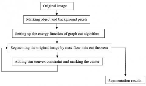
Figure 5 shows the workflow of our vehicle image segmentation algorithm:
Step 1. Input the original vehicle image, mark the object and background, map the image to an S-Tweighted undirected graph, construct the energy function, and design the weights of all edges.
Step 2. Transform the energy function into the minimum cut problem based on the S-T weighted undirected graph, and obtain the initial segmentation results by the max-flow min-cut theorem.
Step 3. Add star convex constrain to vehicle image, manually mark the center, define the prior energy function of star convex, and introduce star convex prior to the energy function of graph cut algorithm, forming the new energy function.
Step 4. Transform the new energy function into the minimum cut problem, reassign the weights to the edges, and re-segment the vehicle image.
Figure 5. The workflow of our algorithm
To verify its effectiveness, our algorithm was applied to segment ordinary vehicle images, shadowed vehicle images, complex background vehicle images, and incomplete vehicle images. The segmentation results were evaluated both qualitatively and quantitatively. The object pixels, background pixels, and star convex center were all marked manually. The four types of images were segmented with and without the star convex constraint. The original images were extracted from BIT-Vehicle Dataset and MIT-CBCL Car Database.
To reflect is superiority, our algorithm was compared with two threshold-based image segmentation algorithms, namely, the Otsu’s method [22] and the traditional graph cut algorithm [12]. For comparison, the gold standard segmentation results were manually marked, laying the basis for quantitative analysis of experimental results.
4.1 Experiment on ordinary vehicle images
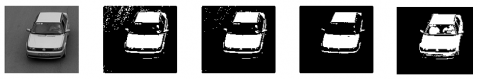
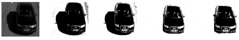
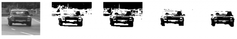
The experimental results on the ordinary vehicle images from BIT-Vehicle Dataset are listed in Figure 6, where column (a) is the original images, column (b) is the segmentation results of Otsu’s method, column (c) is the segmentation results of graph cut algorithm, column (d) is the segmentation results of our algorithm, and (e) is the results of gold standard segmentation.
(1a) Original image; (1b) Result of Otsu’s method; (1c) Result of graph cut algorithm; (1d) Result of our algorithm; (1e) Result of gold standard segmentation
(2a) Original image; (2b) Result of Otsu’s method; (2c) Result of graph cut algorithm; (2d) Result of our algorithm; (2e) Result of gold standard segmentation
(3a) Original image; (3b) Result of Otsu’s method; (3c) Result of graph cut algorithm; (3d) Result of our algorithm; (3e) Result of gold standard segmentation
(4a) Original image; (4b) Result of Otsu’s method; (4c) Result of graph cut algorithm; (4d) Result of our algorithm; (4e) Result of gold standard segmentation
Figure 6. Comparison between segmentation results on ordinary vehicle images from BIT-Vehicle Dataset
As shown in Figure 6, the Otsu’s method and the graph cut algorithm, which is not subjected to star convex constraint, were not as good as our algorithm in details, while our algorithm could highlight the contours of the object. Our algorithm (Figure 6(1d)) could segment the entire vehicle from the image. By contrast, the graph cut brought many burrs and unclear boundaries (Figure 6(1c)), while the Otsu’s method failed to segment the object clearly (Figure 6(1b)). The result of our algorithm in Figure 6(2d) was better than Figure 6(2c) and Figure 6(1c) in object prominence and noise level, and also better than Figure 6(3d) and Figure 6(4d).
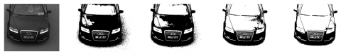
4.2 Experiment on shadowed vehicle images
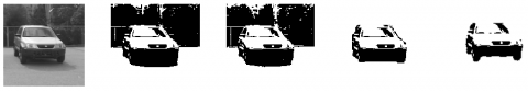
The experimental results on the shadowed vehicle images from BIT-Vehicle Dataset are listed in Figure 7. Our algorithm achieved excellent segmentation effects: the object shapes were effectively identified by the graph cut algorithm coupled with star convex. The vehicles were clearly segmented by our algorithm from all four images. The object shapes were maintained, while the shadows were removed. However, the Otsu’s method and graph cut algorithm could not effectively remove the shadows.
(1a) Original image; (1b) Result of Otsu’s method; (1c) Result of graph cut algorithm; (1d) Result of our algorithm; (1e) Result of gold standard segmentation
(2a) Original image; (2b) Result of Otsu’s method; (2c) Result of graph cut algorithm; (2d) Result of our algorithm; (2e) Result of gold standard segmentation
(3a) Original image; (3b) Result of Otsu’s method; (3c) Result of graph cut algorithm; (3d) Result of our algorithm; (3e) Result of gold standard segmentation
(4a) Original image; (4b) Result of Otsu’s method; (4c) Result of graph cut algorithm; (4d) Result of our algorithm; (4e) Result of gold standard segmentation
Figure 7. Comparison between segmentation results on shadowed vehicle images from BIT-Vehicle Dataset
(1a) Original image; (1b) Result of Otsu’s method; (1c) Result of graph cut algorithm; (1d) Result of our algorithm; (1e) Result of gold standard segmentation
(2a) Original image; (2b) Result of Otsu’s method; (2c) Result of graph cut algorithm; (2d) Result of our algorithm; (2e) Result of gold standard segmentation
(3a) Original image; (3b) Result of Otsu’s method; (3c) Result of graph cut algorithm; (3d) Result of our algorithm; (3e) Result of gold standard segmentation
(4a) Original image; (4b) Result of Otsu’s method; (4c) Result of graph cut algorithm; (4d) Result of our algorithm; (4e) Result of gold standard segmentation
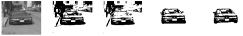
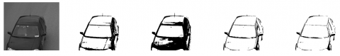
Figure 8. Comparison between segmentation results on complex background vehicle images from MIT-CBCL Car Database
(1a) Original image; (1b) Result of Otsu’s method; (1c) Result of graph cut algorithm; (1d) Result of our algorithm; (1e) Result of gold standard segmentation
(2a) Original image; (2b) Result of Otsu’s method; (2c) Result of graph cut algorithm; (2d) Result of our algorithm; (2e) Result of gold standard segmentation
(3a) Original image; (3b) Result of Otsu’s method; (3c) Result of graph cut algorithm; (3d) Result of our algorithm; (3e) Result of gold standard segmentation
(4a) Original image; (4b) Result of Otsu’s method; (4c) Result of graph cut algorithm; (4d) Result of our algorithm; (4e) Result of gold standard segmentation
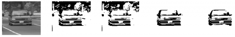
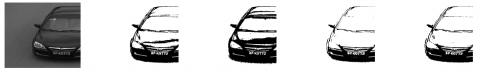
Figure 9. Comparison between segmentation results on complex background vehicle images from BIT-Vehicle Dataset
4.3 Experiment on complex background vehicle images
The vehicle images in Figures 6 and Figure 7 have unified backgrounds. In this subsection, several images are extracted from MIT-CBCL Car Database to verify the effectiveness of our algorithm in segmenting complex background vehicle images. Figure 8 provide experimental results of different image segmentation algorithms on the complex background vehicle images.
As shown in Figure 8, the Otsu’s method and graph cut algorithm performed poorly in segmenting vehicle images with complex background, failing to effectively remove the background. On the contrary, our algorithm segmented the vehicles from these images effectively, despite the interference from the complex background.
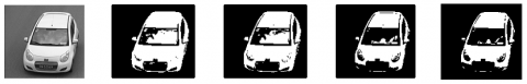
4.4 Experiment on incomplete vehicle images
The experimental results on the incomplete vehicle images from BIT-Vehicle Dataset are listed in Figure 9.
As shown in Figure 9, the Otsu’s method and graph cut algorithm could not effectively remove the details on the edges. Compared with the two methods, our algorithm segmented the incomplete vehicles accurately from all four images, and preserved the shape of the marked objects. The results of our algorithm were closer to the result of gold standard segmentation than those of the Otsu’s method and graph cut algorithm. The excellence of our algorithm demonstrates that the graph cut algorithm, coupled with star convex, can successfully identify the shapes of incomplete vehicles, and proves the universality of star convex.
4.5 Quantitative analysis of experimental data
The experimental results were evaluated qualitatively in the above subsections. This subsection aims to quantitatively compare these results. Usually, quantitative analysis needs to compare the experimental results with the gold standard. However, the gold standard is not established in an absolute sense. Hence, the gold standard segmentation results were manually marked to obtain reliable images of gold standard segmentation.
The experimental results were measured by five metrics, including sensitivity, specificity, precision, accuracy, and mean error rate (MER) [23]:
$Sensitivity=\frac{\left| M\cap G \right|}{\left| G \right|}$ (11)
$Specificity=\frac{\left| \tilde{M}\cap \tilde{G} \right|}{\left| {\tilde{G}} \right|}$ (12)
$\Pr ecision=\frac{\left| M\cap G \right|}{\left| M \right|}$ (13)
$Accuracy=\frac{\left| M\cap G \right|+\left| \tilde{M}\cap \tilde{G} \right|}{N}$ (14)
$MER=\frac{\left| \tilde{M}\cap \left. G \right|+\left| M\cap \left. {\tilde{G}} \right| \right. \right.}{N}$ (15)
where, M is the result of a segmentation algorithm; $\tilde{M}$ is the inverse of the segmentation result; G is the result of gold standard segmentation, i.e. the ideal result; $\tilde{G}$ is the inverse of the result of gold standard segmentation; N is the total number of pixels in the vehicle image.
Tables 1-4 provide the average quantitative evaluation results of the segmentation results of four types of vehicle images.
Table 1. Quantitative evaluation results of ordinary vehicle image experiment
|
Metric Algorithm |
Sensitivity |
Specificity |
Precision |
Accuracy |
MER |
|
Otsu’s method |
0.9015 |
0.9721 |
0.7125 |
0.8926 |
0.1074 |
|
Graph cut algorithm |
0.9236 |
0.9812 |
0.8369 |
0.8951 |
0.1049 |
|
Our algorithm |
0.9554 |
0.9862 |
0.8891 |
0.9030 |
0.0970 |
|
Metric Algorithm |
Sensitivity |
Specificity |
Precision |
Accuracy |
MER |
|
Otsu’s method |
0.7446 |
0.7815 |
0.7968 |
0.7857 |
0.2134 |
|
Graph cut algorithm |
0.7951 |
0.8126 |
0.7693 |
0.7963 |
0.2037 |
|
Our algorithm |
0.9687 |
0.9772 |
0.9165 |
0.9328 |
0.0672 |
|
Metric Algorithm |
Sensitivity |
Specificity |
Precision |
Accuracy |
MER |
|
Otsu’s method |
0.7559 |
0.7610 |
0.6523 |
0.5415 |
0.4585 |
|
Graph cut algorithm |
0.7996 |
0.7812 |
0.7184 |
0.5658 |
0.4342 |
|
Our algorithm |
0.9868 |
0.9635 |
0.8857 |
0.9256 |
0.0744 |
|
Metric Algorithm |
Sensitivity |
Specificity |
Precision |
Accuracy |
MER |
|
Otsu’s method |
0.9021 |
0.9613 |
0.8210 |
0.8837 |
0.1296 |
|
Graph cut algorithm |
0.9188 |
0.9829 |
0.8419 |
0.9106 |
0.1155 |
|
Our algorithm |
0.9625 |
0.9910 |
0.8997 |
0.9357 |
0.0796 |
According to the features of vehicle images (e.g. shadow and complex background), this paper introduces the shape features of the vehicle into the graph cut algorithm, producing a novel vehicle image segmentation algorithm. The proposed algorithm was applied to segment vehicle images in different scenarios, aiming to constrain the shape of segmented results. Experimental results show that our algorithm outperformed the Otsu’s method and graph cut algorithm in segmenting complex background vehicle images, shadowed vehicle images, and incomplete vehicle images. Our algorithm is an effective and accurate way to remove vehicle shadows and background.
This paper was supported by National Natural Science Foundation of China (Grant No.: 61876184), Natural Science Foundation of Anhui Province (Grant No.: 1708085QF157, 1908085QF287), Support Program for Excellent Young Talents in Universities, Anhui Province (Grant No.: gxyq2017050), and Natural Science Foundation for Universities, Anhui Province (Grant No.: KJ2020A0090, KJ2020A0113).
[1] Gonzalez, R.C., Woods, R.E. (2002). Digital Imaging Processing. Prentice Hall: New York, NY, USA, 2002.
[2] Pal, N.R., Pal, S.K. (1993). A review on image segmentation techniques. Pattern Recognition, 26(9): 1277-1294. https://doi.org/10.1016/0031-3203(93)90135-J
[3] Boykov, Y., Jolly, M.P. (2001). Interactive graph cuts for optimal boundary and region segmentation of objects in N-D images. In: Proceedings of the 8th IEEE International Conference on Computer Vision. Vancouver, Canada: IEEE, pp. 105-112. https://doi.org/10.1109/ICCV.2001.937505
[4] Rother, G., Kolmogorov, V., Blake, A. (2004). “GrabCut”-Interactive Foreground Extraction using Iterated Graph Cuts. ACM Transactions on Graphics, 23(4): 309-314. https://doi.org/10.1145/1015706.1015720
[5] An, N.Y., Pun, C.M. (2013). Iterated graph cut integrating texture characterization for interactive image segmentation. International Conference Computer Graphics, Imaging and Visualization, Macau, pp. 79-83. https://doi.org/10.1109/CGIV.2013.34
[6] Hou, Y. (2011). Research on image segmentation based on graph theory. Xian. Shanxi. Xidian University. CNKI: CDMD:1.1011.200474
[7] Pi, Z.M. (2013). A study on image segmentation algorithm based on depth information. Anhui Hefei: University of Science and Technology of China.
[8] Gazcon, N.F., Chesñevar, C.L., Castro, S.M. (2012). Automatic vehicle identification for Argentinean plates using intelligent template matching. Pattern Recognition Letters, 33(9): 1066-1074. https://doi.org/10.1016/j.patrec.2012.02.004
[9] Chang, J.C., Chou, T. (2014). Iterative graph cuts for image segmentation with a nonlinear statistical shape prior. Computer Vision and Pattern Recognition, New York, 49: 87-97. https://doi.org/10.1007/s10851-013-0440-9
[10] Wang, H., Zhang, H., Ray, N. (2013). Adaptive shape prior in graph cut image segmentation. Pattern Recognition, 46(5): 1409-1414. 10.1109/ICIP.2010.5653335
[11] Chang, J., Chou, T., Brennan, K. (2011). Tracking monotonically advancing boundaries in image sequences using graph cuts and recursive kernel shape priors. IEEE Transactions Medical Imaging, 13(5): 1008-1020. https://doi.org/10.1109/TMI.2011.2178122
[12] Boykov, Y., Veksler, O. (2006). Graph cuts in vision and graphics: Theories and applications. Handbook of Mathematical Models in Computer Vision. New York: Springer, 79-96. https://doi.org/10.1007/0-387-28831-7_5
[13] Tian, Y.S., Yap, K.H., He, Y. (2012). Vehicle license plate super-resolution using soft learning prior. Multimedia Tools and Applications, 60(3): 519-535. https://doi.org/10.1007/s11042-011-0821-2
[14] Ghanem, B., Ahuja, N. (2010). Dinkelbach NCUT: an efficient frame work for solving normalized cuts problems with priors and convex constraints. International Journal of Computer Vision, 89(1): 40−55. https://doi.org/10.1007/s11263-010-0321-2
[15] Candemir, S., Akgul, Y.S. (2010). Adaptive regularization parameter for graph cut segmentation. In: Proceedings of the 7th International Conference on Image Analysis and Recognition. Povoa de Varzim, Portugal: Springer, pp. 117-126. https://doi.org/10.1007/978-3-642-13772-3_13
[16] Le, T.H., Jung, S.W., Choi, K.S., Ko, S.J. (2010). Image segmentation based on modified graph-cut algorithm. Electronics Letters, 46(16): 1121-1122. https://doi.org/10.1049/el.2010.1692
[17] Tao, W.B., Jin, H. (2007). A new image thresholding method based on graph spectral theory. Chinese Journal of Computers, 30(1): 110-119.
[18] Veksler, O. (2008). Star shape prior for graph cut image segmentation. In: Proceedings of the 10th European Conference on Computer Vision. Marseille, France: Springer, pp. 454-467. https://doi.org/10.1007/978-3-540-88690-7_34
[19] Gulshan, V., Rother, C., Criminisi, A., Blake, A., Zisserman, A. (2010). Geodesic Star Convexity for Interactive Image Segmentation. 2010 IEEE Computer Society Conference on Computer Vision and Pattern Recognition, San Francisco, CA, USA, pp. 3129-3136. https://doi.org/10.1109/CVPR.2010.5540073
[20] Veksler, O. (2008). Star shape prior for graph cut image segmentation. European Conference on Computer Vision, pp. 454-467. https://doi.org/10.1007/978-3-540-88690-7_34
[21] Shi, J., Malik, J. (2000). Normalized cuts and image segmentation. IEEE Transactions on Pattern Analysis and Machine Intelligence, 22(8): 888-905. https://doi.org/10.1109/34.868688
[22] Wang, R., Wu, H., Fang, S., Yang, W. (2010). A new adaptive two-dimensional Otsu image segmentation algorithm research. Journal of University of Science and Technology of China, 40: 841-847.
[23] Liao, X., Xu, H., Zhou, Y., Li, K.Q., Tao, W.B., Guo, Q.J., Liu, L.M. (2014). Automatic Image Segmentation using Salient Key Point Extraction and Star Shape Prior. Signal Processing, 105(12): 122-136. https://doi.org/10.1016/j.sigpro.2014.04.035