Baohai Yang
© 2020 IIETA. This article is published by IIETA and is licensed under the CC BY 4.0 license (http://creativecommons.org/licenses/by/4.0/).
OPEN ACCESS
Currently, many adaptive filtering algorithms are available for the non-Gaussian environment, namely, least mean square (LMS) algorithm, recursive least square (RLS) algorithm, least mean fourth (LMF) algorithm, and subspace minimum norm (SMN) algorithm. Most of them can converge to the steady-state, but face various constraints in the presence of alpha (α)-stable noises. To solve the problem, this paper aims to develop an adaptive filtering algorithm for non-Gaussian signals in α-stable distribution, drawing on the merits of existing adaptive filtering algorithms. Firstly, the authors introduced the theory of α-stable distribution, the central limit theorem and fractional lower-order statistics (FLOS). Next, two classic adaptive filtering algorithms, RLS and LMS, were summarized, and compared through tests. On this basis, the FLOS-SMN algorithm was designed in the light of the features of the LMS and the SMN, which applies to the filtering of non-Gaussian signals in α- stable distribution. Finally, the proposed algorithm was proved as faster, more stable and more adaptable than the traditional method.
Alpha (α)-stable distribution, non-Gaussian distribution, fractional lower-order statistics (FLOS), adaptive filtering algorithm, least mean square (LMS), subspace minimum norm (SMN) algorithm
With strong impact features, human signals (e.g. underwater signals, atmospheric signals, and biomedical signals) are clearly different from traditional Gaussian signals. The distribution of these non-Gaussian signals, featuring a finite variance and long tails, can be described as processes with a finite or infinite variance. In engineering applications, non-Gaussian signals often obey alpha (α)-stable distribution [1-8].
In general, non-Gaussian signals are processed based on higher-order statistics (HOS) or fractional lower-order statistics (FLOS) [9-12]. If these signals are incorrectly assumed to satisfy Gaussian distribution, the filter will perform poorly or cease to be effective [13], because these signals obey α-stable distribution rather than Gaussian distribution.
In Gaussian distribution model, the observations are treated as elements in a Hilbert space, and the second-order statistics is taken as the optimal filtering criterion. In α-stable distribution model, the observations are treated as elements in Banach space (1≤α<2) or metric space (0<α<1). The two spaces differ greatly from the Hilbert space in properties.
With the growing number of samples, the variance of Gaussian signals converges, but that of α-stable signals does not converge. For signals in α-stable distribution, the second-order statistics is not a suitable optimal filtering criterion, and the minimum mean square error (MMSE) criterion is not sufficiently significant [14-16].
In light of the above, this paper proposes an adaptive filtering algorithm for non-Gaussian signals in α-stable distribution, based on the least mean square (LMS) algorithm and the subspace minimum norm (SMN) algorithm.
2.1 Concept of α- stable distribution
For any random variable X, if there exists α∈(1, 2) satisfying:
$C^{\alpha}=A^{\alpha}+B^{\alpha}$ (1)
Then, X is an α-stable random variable, where α is the characteristic index. Thus, the α-stable distribution can be defined as: the random variable X obeys the stable distribution, if 1<α≤2, γ≤0 and -1<β≤1, if parameter a is a real number, and if the characteristic functions satisfy:
$\phi(u)=\exp \left\{j a u-\gamma|u|^{\alpha}[a+j \beta \operatorname{sign}(t) \varpi (u, \alpha)]\right\}$ (2)
where, ω(u,α) and sign(u) can be respectively expressed as:
$\omega(u, \alpha)=\left\{\begin{array}{l}\frac{\pi}{2} \log |u|, \alpha=1 \\ \tan \frac{\alpha \pi}{2}, \alpha \neq 1\end{array}\right.$ (3)
$\operatorname{sign}(u)=\left\{\begin{array}{l}1, u>0 \\ 0, t=0 \\ -1, u<0\end{array}\right.$ (4)
where, β is the symmetry coefficient that expresses the slope of qualifiers distribution; γ, similar to the variance in Gaussian distribution, illustrates the dispersion of qualifiers distribution; u is the position parameter, corresponding to the mean or median.
The characteristic index 0<α≤2 determines the intensity of the pulse. The smaller the α value, the heavier the tail of distribution; the inverse is also true. If α=0, formula (2) can be rewritten as φ(u)=exp{jαu-σ2|u|2}, which is a special case of stable Gaussian distribution. If α=1 and β=0, formula (2) is a Cauchy distribution [17]. If α∈(0, 2], formula (2) becomes a non-Gaussian α-stable distribution, which has a greater impact than the Gaussian distribution.
Gaussian distribution is actually a special case of α-stable distribution. If 1<α<2, the α-stable distribution can be called a Francoise lower-order alpha (FLOA) [18-19]; if β=0, u=0 and γ=1, the α-stable distribution can be called a symmetry α-stable (SαS) distribution; If α=2, the distribution becomes a Gaussian distribution.
2.2 Central limit theorem
The central limit theorem holds that: if xi is independent and identically distributed with finite variance, the limit distribution is Gaussian distribution. The main difference between the α-stable distribution and the Gaussian distribution lies in the tail. The former has an algebraic tail, while the latter, an exponential tail.
2.3 FLOS
In recent years, the HOS has been widely adopted for signal analysis, i.e. the effective information is extracted from third- or fourth-order statistics. On this basis, the statistics lower than the second-order, i.e. the FLOS, was developed for signal analysis [20].
Let E[X2] be the second-order moment of the FLOS X. Then, the fractional-lower order (FLO) moment E[|X|P] (0<p<2) for α-stable distribution can be defined as:
$E\left[|X|^{P}\right]=\left\{\begin{array}{cl}C(p, a) \gamma^{\frac{p}{\alpha}}, 0<p \leq \alpha \\ \infty & , p \geq a\end{array}\right.$ (5)
where, X is a random process in SαS distribution; α (α=0) is the position parameter; γ is the dispersion coefficient; C(p, α) is a function related to p and a but not to X.
2.4 Negative moments
Studies have shown that SαS random variable distribution might have finite negative moments:
$E\left(|x|_{p}\right)=c(p, \alpha) \gamma^{\frac{p}{\alpha}},-1<p<\alpha$ (6)
The adaptive filtering algorithm is defined as a filter algorithm capable of adjusting and tracking its own parameters, without knowing the statistical properties of input signals and noises [21-22].
3.1 LMS algorithm
The LMS algorithm replaces the mean squared error (MSE) E[e2(n)] with the instantaneous squared value of output error |e(n)|2 [23]. In each iteration, the gradient estimation takes the following form:
$\hat{\nabla} n=\frac{\partial}{\partial w_{n}}|e(n)|^{2}=\frac{\partial}{\partial w_{n}}\left[|d(n)|^{2}+w^{T}(n) \mathbf{x}_{M}^{T}(n) w(n)-2 \operatorname{Re}\left(d(n) \mathbf{x}_{M}^{T}(n) w(n)\right)\right]$
$=2 \mathbf{x}_{M}(n) \mathbf{x}_{M}^{T} w(n)-2 d(n) \mathbf{x}_{M}(n)=-2 e(n) \mathbf{x}_{M}(n)$ (7)
On this basis, the iterative formula of the LMS algorithm can be derived as:
$\mathbf{w}(n+1)=\mathbf{w}(n)-\mu e(n) \mathbf{X}_{m}(n)$ (8)
Under normal circumstances, the LMS algorithm is highly adaptable. However, the step length μ is difficult to determine, and the convergence is relatively slow [24, 25]. In the basic LMS algorithm, the value of μ usually remains constant, which is obviously not suitable for the iterative process. This gives rise to the normalized least mean square (NLMS) algorithm [26, 27], an LMS algorithm with variable step size.
In the NLMS algorithm, the step length μ varies with the elapse of time [28]:
$\mu(n)=\frac{\alpha}{\beta+\mathbf{X}_{M}^{T}(n) \mathbf{X}_{M}(n)}$ (9)
The weight vector is updated by:
$w(n)=w(n-1)+\frac{1}{\lambda+\left\|x_{M}(n)\right\|_{1}} \operatorname{sgn}(e(n)) x_{M}(n)$ (10)
This constitutes the so-called symbol error NLMS algorithm [29].
3.2 RLS algorithm
Compared with the LMS algorithm, the RLS algorithm has a fast tracking speed, which is an important capability for time-varying channels. Since the measurable data may have variable length [30], the minimized cost can be represented as a cost function J(n):
$\mathbf{J}(n)=\sum_{i=1}^{n} \lambda^{n-i}|\xi(i)|^{2}=\sum_{i=1}^{n} \lambda^{n-i}\left|d(i)-\mathbf{W}^{T}(n) \mathbf{X}_{M}(i)\right|^{2}$ (11)
where, n is the variable length; ξ(i) can be expressed as:
$e(i)=d(i)-y(i)=d(i)-\mathbf{w}^{T}(n) \mathbf{x}_{M}(i)$ (12)
XM(i) is the tapping input vector:
$\mathbf{x}_{M}(i)=[x(i), x(i-1), \ldots, x(i-M+1)]^{T}$ (13)
W(n) is weight vector at time n:
$\mathbf{w}(n)=\left[w_{0}(n), w_{1}(n), \ldots, w_{M-1}(n)\right]^{T}$ (14)
Note that the tap weights remain the same in the observation interval 1≤i≤n defined by the cost function J(n).
The weighting factor β (n, i) was introduced to make the filter track the changes of observed data under non-stationary environment [31]:
$\beta(n, i)=\lambda^{n-i}, i=1,2, \cdots n$ (15)
The weighting factor should satisfy:
$0<\beta(n, i) \leq 1, i=1,2, \ldots, n$ (16)
The cost function Jw(n) can be described as the sum of the weighted sum of squared errors and the regularization term.
$\mathbf{J}_{w}(n)=\sum_{i=1}^{n} \lambda^{n-i}|\xi(i)|^{2}+\delta \lambda^{n}\|\mathbf{w}(n)\|^{2}$ (17)
The weighted sum of squared errors can be expressed as:
$\sum_{i=1}^{n} \lambda^{n-i}|\xi(i)|^{2}=\sum_{i=1}^{n} \lambda^{n-i}\left|d(i)-\mathbf{w}^{T}(n) \mathbf{X}_{M}(i)\right|^{2}$ (18)
Depending on the input data, the weighted sum of squared errors reflects the relationship between the expected response d(i) and the actual response y(i) of the filter:
$y(i)=\mathbf{W}^{T}(n) \mathbf{X}_{M}(i)$ (19)
The regularization term can be expressed as:
$\delta \lambda^{n}\|\mathbf{w}(n)\|^{2}=\delta \lambda^{n} \mathbf{w}^{T}(n) \mathbf{w}(n)$ (20)
where, the regularization parameter δ is a positive real number. It can be seen that regularization only depends on W(n). To solve the problem of least squares regression, smoothing should be considered in the regularization process [32].
Despite its fast convergence, the RLS algorithm faces an insufficient stability, possible divergence, and complex computing, failing to output ideal results [33]. If H-1 is not positive definite, the RLS algorithm cannot be updated; if when λ<1, the algorithm will diverge.
3.3 Comparison between RLS and LMS algorithms
The structure of the LMS filter is explained in Figure 1 below.
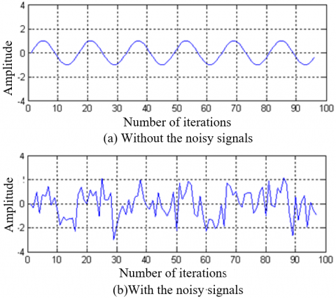
The noisy input signals can be expressed as:
$x(n)=s(n)+v(n)$ (21)
where, s(n)=sin[2πnf/fs] (f=50, fs=16, n=0, 1, …, N-1; N=96); the mean value of v(n) is zero. The input signals contain Gaussian distribution with the variance of 1. The signal waves of the LMS filter with and without the noisy signals are displayed in Figure 2.
Figure 1. The structure of the LMS filter
Figure 2. The signal waves of the LMS filter with and without the noisy signals
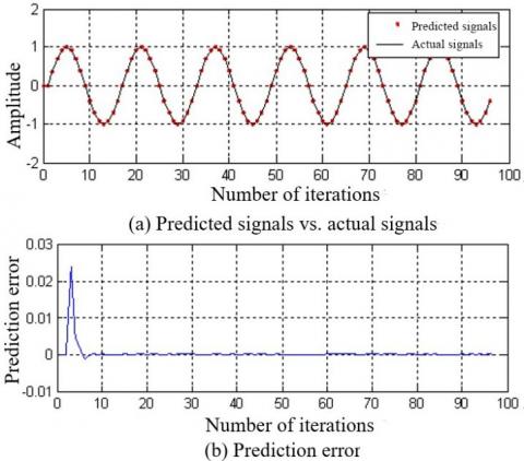
The LMS and RLS algorithms were simulated separately to compare their features. First, the filter length and step length of the LMS algorithm were set as M=32 and μ=32, respectively. The signals predicted by the LMS and the actual signals are compared in Figure 3(a), and the prediction error of the LMS is shown in Figure 3(b). Obviously, the LMS algorithm could effectively predict the actual signals after a period of time.
Next, the RLS algorithm was adopted with the forgetting factor λ=0.48. The other parameters were the same as the LMS algorithm. The filtering performance of the RLS algorithm is presented in Figure 4 below.
According to the comparison between Figures 3 and 4, it took only 10 iterations for the RLS algorithm, but 100 iterations for the LMS algorithm, to reach the steady-state. Obviously, the RLS converged much faster than the LMS. However, the fast convergence was realized with a high computing complexity and instability. By contrast, the LMS algorithm is easy to implement and stable in performance. But this algorithm is too sensitive to ratio of the maximum eigenvalue to the minimum eigenvalue. Therefore, this paper attempts to design a new filtering algorithm that combines the merits of the LMS and other algorithms.
Figure 3. The filtering performance of the LMS algorithm
Figure 4. The filtering performance of the RLS algorithm
4.1 Adaptive system identification model
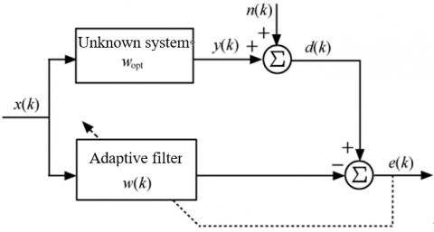
In our adaptive system identification model (Figure 5), the input signals can be described as Xk=[x(k),x(k-1),…,x(k-N+1)]T, where N is the order of the filter. Let n be the length of input sequence, wk is the weight vector of adaptive filter, and nk be the α-stable distribution noises of input signals [34]. As shown in Figure 5, e(k) can be expressed as:
$e(k)=d(k)-\mathbf{X}(k)^{T} w(k)=X_{k}^{T} w_{o p t}+n(k)-X_{k}^{T} w(k)=\left[w_{o p t}-w(k)\right]^{T} \mathbf{X}(k)+n(k)$ (22)
Figure 5. Adaptive system identification model
4.2 Algorithm implementation
In this paper, the LMS algorithm is improved under non-Gaussian α-stable conditions, and verified through simulation [35].
Taking J(k)=E|e(k)|2 as the cost function, the LMS algorithm has the following iterative formula:
$\mathbf{w}(k+1)=\mathbf{w}(k)+\mu e(k) x(k)$ (23)
The least-mean-fourth (LMF) algorithm takes J(k)=E|e(k)|4 as its cost function. The relationship between LMS and LMF algorithms can be summarized as an SMN algorithm with the cost function:
$J(k)=\frac{1}{2} \lambda E\left|e(k)\right|^{2}+\left(\frac{1}{2}\right)^{2} \lambda^{2} E|e(k)|^{4}$
$+\left(\frac{1}{2}\right)^{3} \lambda^{3} E|e(k)|^{8}+\ldots+\left(\frac{1}{2}\right)^{n} \lambda^{n} E|e(k)|^{2^{i}}=\sum_{i=1}^{n}\left(\frac{1}{2}\right)^{i} \lambda^{i}\left\{E[|e(k)|]^{|\rho|}\right\}^{2^{i}}$ (24)
The iterative formula of the LMF algorithm can be expressed as:
$\mathbf{w}(k+1)=\mathbf{w}(k)+\mu\left\{\lambda E|e(k)|+\lambda^{2} E|e(k)|^{3}\right.$
$\left.+\lambda^{3} E|e(k)|^{7}+\ldots .+\lambda^{n} E|e(k)|^{2^{n}-1}\right\} x(k)=\mathbf{w}(k)+\mu\left[\sum_{i=1}^{n} \lambda^{(i-1)} e(k)^{2 i-1}\right] x(k)$ (25)
where, 0≤λ≤1 is the hybrid parameter. Under Gaussian noises, the second moment E|e(k)|2, the fourth moment E|e(k)|4 and the 2n-th moment E|e(k)|2n of the instantaneous error e(k) have limited values. Under SαSG noises, the three moments have no finite values, and the iterative formula (25) is no more applicable. In this case, e(k) [36] can be replaced by seeking for a convergent expression.
The next step is to make the SMN algorithm, which only applies to Gaussian noises, suitable for the FLOS distribution through expansion [37]. Under α-stable noises, if x=y, the FLO covariance can be defined as the FLO auto-covariance. From the properties of the FLOS, we have:
$F L O C(X, X)=E\left\{X^{\mathrm{<P>}} X^{* \mathrm{<P>}}\right\}=E\left\{|X|^{2 \mathrm{<P>}}\right\}=E\left\{\left.X^{\mathrm{<P>}}\right|^{2}\right\}$ (26)
If 0<P≤α, the P-order moment E[|X)|P]<∞. Then, 0<P≤α/2, 0<2P≤α and:
$E\left[\left|X^{<P>}\right|^{2}\right]=E\left[|X|^{P-1} X^{*}\left(|X|^{P-1} X^{*}\right)^{*}\right]=E\left[|X|^{2 P}\right]<\infty$ (27)
Similarly, if 0<P≤α/2n, then 0<2nP≤α and:
$E\left[\left|X^{<P>}\right|^{2^{n}}\right]=E\left[|X|^{2^{n} P}\right]<\infty$ (28)
Replacing e(k) in formula (25) with e(k)<P>, a new algorithm suitable for SαSG noises can be obtained, which is called FLOS-SMN [38]. In the new algorithm, the cost function can be expressed as:
$J(k)=\sum_{i=1}^{n}\left(\frac{1}{2}\right)^{i} \lambda^{(i-1)}\left\{E[|x|]^{<p>}\right\}^{2 i}$ (29)
Taking the derivative of w(k), the gradient can be estimated as:
$\partial\left\{\sum_{i=1}^{n}\left(\frac{1}{2}\right)^{i} \lambda^{(i-1)}\left\{E[|x|]^{\langle p\rangle}\right\}^{2 i}\right\} / \partial[w(k)]$
$=-p \sum_{i=1}^{n} \lambda^{(i-1)}\left\{e(k)^{\langle p\rangle}\right\}^{\left(2^{i}-1\right)} \cdot|e(k)|^{(p-1)} x(k)$ (30)
Thus, the iterative formula can be obtained as:
$\mathbf{w}(k+1)=\mathbf{w}(k)+\mu \sum_{i=1}^{n} \lambda^{i}\left\{[e(k)]^{(p-1)}\right\}^{2^{i}} \operatorname{sign}[e(k)] \cdot x(k)$ (31)
where, 0≤λ≤1 is hybrid parameter; μ is the step length; 0<P≤α/2n; α(α<2) is the characteristic index of α-stable distribution noises.
Suppose the unknown system in Figure 5 is wopt=[1, a1,…, a10]=[1 2 3 4 5 6 5 4 3 2 1]. The input signals can be defined as:
$x(k)=\sin [2 \pi \cdot 0.02 \cdot(0: \mathrm{k})]$
$y(k)+a_{1} y(k-1)+\cdots+a_{8} y(k-8)+a_{9} y(k-9)+a_{10} y(k-10)=x(k)$ (32)
Let n(k) be independent additive SαSG noises:
$d(k)=y(k)+n(k)=X(k)^{T} w_{o p t}+(1 / A) \mathrm{S} \alpha \mathrm{SG}\left(\alpha, \gamma_{\mathrm{S} \alpha \mathrm{SG}}, \gamma_{\mathrm{G}}\right)$ (33)
where, k=1, 2, …, N (N is the sequence length). If N=500 and γSαSG=2γG=γ=1, the mixed signal-to-noise ratio MSNRSαSG can be defined as:
MSNR $_{\mathrm{S} \alpha \mathrm{SG}}=10 \log _{10}\left(\sigma_{S}^{2} / \gamma\right)$
$=10 \log _{10}\left(\frac{1}{\gamma N} \sum_{n=1}^{N}\left|s_{i}(n)\right|^{2}\right)$
$\quad=10 \log _{10}\left(\frac{1}{N} \sum_{n=1}^{N}\left|s_{i}(n)\right|^{2}\right)$ (34)
Then, the signal magnitude can be derived from MSNRSαSG:
$A=10^{\frac{M S N R_{\text {sasg}}}{10}} / \frac{1}{N} \sum_{n=1}^{N}\left|s_{i}(n)\right|^{2}$ (35)
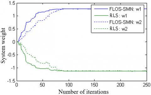
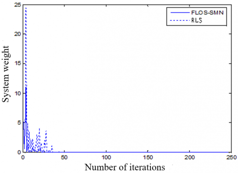
Next, the FLOS-SMN was compared with the RLS with the initial weight vector w0=0, step length μ=0.06, and K=200. The system weight curves of both algorithms are compared in Figure 6 below.
Figure 6. Comparison of system weight curves
As shown in Figure 6, the system weights of both algorithms converged quickly and smoothly to the steady-state values. However, the system weights of the FLOS-SMN were much larger than those of the RLS.
Taking hybrid parameter λ=0.5, percentage of α-stable distribution noises p=1.2 and the steady state error power as Pε, the equivalent convergence factors (μ1 and μ2) of the two algorithms were obtained.
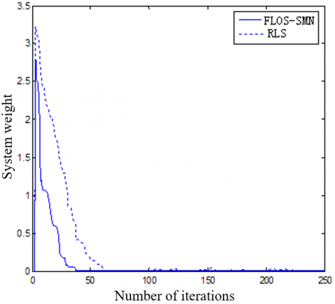
Next, the adaptive filter coefficients were initialized as w(k)=[1 2 3 4 5 6 5 4 3 2 1], and the SNR was set to 2dB. Then, both FLOS-SMN and RLS were iterated adaptively. The filtering performance of the two algorithms is compared in Figures 7 and 8. It can be seen that the MSE learning curve of the FLOS-SMN converged to the steady-state earlier, and had fewer jitters than the RLS.
Figure 7. Comparison of MSE learning curves
Figure 8. Comparison of vector learning curves
Besides the common Gaussian noises, the α-stable noises are also a hot topic in signal processing. This paper mainly designs and implements an adaptive filtering algorithm for signals obeying the α-stable distribution. Firstly, the theory on α-stable distribution was thoroughly reviewed. Then, adaptive filters like the RLS and LMS were introduced in details, and compared through tests. Based on the LMS algorithm, the authors developed the SMN algorithm, and defined its scope of application: second-order noise distribution. Thus, the SMN algorithm was improved into the FLOS-SMN algorithm, to suit the noises obeying the FLO distribution. Finally, the proposed algorithm was compared with the traditional RLS algorithm in experiments. The comparison shows that our algorithm achieved faster computing speed, converged to the steady-state earlier, and had fewer jitters than the RLS.
This work was supported in part by the National Science Foundation of Jiangxi Province under Grant 20192BAB207002, in part by the Science and Technology Project of Jiangxi Provincial Health Commission under Grant 20183016, in part by the Science Foundation of Guangxi Normal University for Nationalities under Grant 2019FG008.
[1] Aalo, V.A., Ackie, A.B.E., Mukasa, C. (2019). Performance analysis of spectrum sensing schemes based on fractional lower order moments for cognitive radios in symmetric α-stable noise environments. Signal Processing, 154: 363-374. https://doi.org/10.1016/j.sigpro.2018.09.025
[2] Langhammer, L., Dvorak, J., Sotner, R., Jerabek, J. (2017). Electronically tunable fully-differential fractional-order low-pass filter. Elektronika ir Elektrotechnika, 23(3): 47-54. https://doi.org/10.5755/j01.eie.23.3.18332
[3] LI, B., Ma, H.S., Liu, M.Q. (2014). Carrier frequency estimation method of time-frequency overlapped signals with alpha-stable noise. Journal of Electronics & Information Technology, 36(4): 868-874. https://doi.org/10.3724/SP.J.1146.2013.00827
[4] Chen, Z., Geng, X., Yin, F. (2016). A harmonic suppression method based on fractional lower order statistics for power system. IEEE Transactions on Industrial Electronics, 63(6): 3745-3755. https://doi.org/10.1109/TIE.2016.2521347
[5] Long, J., Wang, H., Li, P., Fan, H. (2017). Applications of fractional lower order time-frequency representation to machine bearing fault diagnosis. IEEE/CAA Journal of Automatica Sinica, 4(4): 734-750. https://doi.org/10.1109/JAS.2016.7510190
[6] Duan, X., Qi, P., Tian, Z. (2016). Registration for variform object of remote-sensing image using improved robust weighted kernel principal component analysis. Journal of the Indian Society of Remote Sensing, 44(5): 675-686. https://doi.org/10.1007/s12524-015-0545-2
[7] Tzagkarakis, G., Nolan, J.P., Tsakalides, P. (2018). Compressive sensing using symmetric alpha-stable distributions for robust sparse signal reconstruction. IEEE Transactions on Signal Processing, 67(3): 808-820. https://doi.org/10.1109/TSP.2018.2887400
[8] Wang, Y., Qi, Y., Wang, Y., Lei, Z., Zheng, X., Pan, G. (2016). Delving into α-stable distribution in noise suppression for seizure detection from scalp EEG. Journal of Neural Engineering, 13(5): 056009. https://doi.org/10.1088/1741-2560/13/5/056009
[9] Bozovic, R., Simic, M. (2019). Spectrum sensing based on higher order cumulants and kurtosis statistics tests in cognitive radio. Radioengineering, 29(2): 464-472. https://doi.org/10.13164/re.2019.0464
[10] Lyka, E., Coviello, C.M., Paverd, C., Gray, M.D., Coussios, C.C. (2018). Passive acoustic mapping using data-adaptive beamforming based on higher order statistics. IEEE Transactions on Medical Imaging, 37(12): 2582-2592. https://doi.org/10.1109/TMI.2018.2843291
[11] Chen, P., Liu, L., Wang, X., Chong, J., Zhang, X., Yu, X. (2017). Modulation model of high frequency band radar backscatter by the internal wave based on the third-order statistics. Remote Sensing, 9(5): 501. https://doi.org/10.3390/rs9050501
[12] Xu, Q., Liu, K. (2019). A new feature extraction method for bearing faults in impulsive noise using fractional lower-order statistics. Shock and Vibration, 1-13. https://doi.org/10.1155/2019/2708535
[13] Zhong, X., Cai, K., Chen, P., Mei, Z. (2020). Design of protograph codes for additive white symmetric alpha-stable noise channels. IET Communications, 14(1): 105-110. https://doi.org/10.1049/iet-com.2019.0332
[14] Shao, M., Nikias, C. L. (1993). Signal processing with fractional lower order moments: Stable processes and their applications. Proceedings of the IEEE, 81(7): 986-1010. https://doi.org/10.1109/5.231338
[15] Said, L.A., Ismail, S.M., Radwan, A.G., Madian, A.H., El-Yazeed, M.F.A., Soliman, A.M. (2016). On the optimization of fractional order low-pass filters. Circuits, Systems, and Signal Processing, 35(6): 2017-2039. https://doi.org/10.1007/s00034-016-0258
[16] Mahata, S., Saha, S.K., Kar, R., Mandal, D. (2018). Optimal design of fractional order low pass Butterworth filter with accurate magnitude response. Digital Signal Processing, 72: 96-114. https://doi.org/10.1016/j.dsp.2017.10.001
[17] Talebi, S.P., Werner, S., Mandic, D.P. (2018). Distributed adaptive filtering of α-stable signals. IEEE Signal Processing Letters, 25(10): 1450-1454. https://doi.org/10.1109/LSP.2018.2862639
[18] Long, J., Wang, H., Zha, D., Li, P., Xie, H., Mao, L. (2017). Applications of fractional lower order S transform time frequency filtering algorithm to machine fault diagnosis. PloS One, 12(4): e0175202. https://doi.org/10.1371/journal.pone.0175202
[19] Kubanek, D., Freeborn, T. (2018). (1+ α) fractional-order transfer functions to approximate low-pass magnitude responses with arbitrary quality factor. AEU-International Journal of Electronics and Communications, 83: 570-578. https://doi.org/10.1016/j.aeue.2017.04.031
[20] Li, D., Liu, J., Zhao, J., Wu, G., Zhao, X. (2017). An improved space-time joint anti-jamming algorithm based on variable step LMS. Tsinghua Science and Technology, 22(5): 520-528. https://doi.org/10.23919/TST.2017.8030541
[21] Saeed, M.O.B. (2017). LMS-based variable step-size algorithms: A unified analysis approach. Arabian Journal for Science and Engineering, 42(7): 2809-2816. https://doi.org/10.1007/s13369-017-2453-y
[22] Eweda, E., Bershad, N.J., Bermudez, J.C.M. (2018). Stochastic analysis of the LMS and NLMS algorithms for cyclostationary white Gaussian and non-Gaussian inputs. IEEE Transactions on Signal Processing, 66(18): 4753-4765. https://doi.org/10.1109/TSP.2018.2860552
[23] Piggott, M.J., Solo, V. (2016). Diffusion LMS with correlated regressors I: Realization-wise stability. IEEE Transactions on Signal Processing, 64(21): 5473-5484. https://doi.org/10.1109/TSP.2016.2576426
[24] Mandal, A., Mishra, R., Kaushik, B.K., Rizvi, N.Z. (2016). Design of LMS adaptive radar detector for non-homogeneous interferences. IETE Technical Review, 33(3): 269-279. https://doi.org/10.1080/02564602.2015.1093436
[25] Shi, L., Zhao, H. (2016). Variable step-size distributed incremental normalised LMS algorithm. Electronics Letters, 52(7): 519-521. https://doi.org/10.1049/el.2015.3882
[26] Pauline, S.H., Samiappan, D., Kumar, R., Anand, A., Kar, A. (2020). Variable tap-length non-parametric variable step-size NLMS adaptive filtering algorithm for acoustic echo cancellation. Applied Acoustics, 159: 107074. https://doi.org/10.1016/j.apacoust.2019.107074
[27] Shah, S.M., Samar, R., Khan, N.M., Raja, M.A.Z. (2017). Design of fractional-order variants of complex LMS and NLMS algorithms for adaptive channel equalization. Nonlinear Dynamics, 88(2): 839-858. https://doi.org/10.1007/s11071-016-3279-y
[28] Matsuo, M.V., Kuhn, E.V., Seara, R. (2019). Stochastic analysis of the NLMS algorithm for nonstationary environment and deficient length adaptive filter. Signal Processing, 160: 190-201. https://doi.org/10.1016/j.sigpro.2019.02.001
[29] Yan, P., Zhao, Z., Shang, J., Zhao, Z. (2013). Variable memory length LMP algorithm of second-order Volterra filter. Jisuanji Gongcheng yu Yingyong(Computer Engineering and Applications), 49(3): 121-125.
[30] Rastegarnia, A., Khalili, A., Bazzi, W.M., Sanei, S. (2016). An incremental LMS network with reduced communication delay. Signal, Image and Video Processing, 10(4): 769-775. https://doi.org/10.1007/s11760-015-0809-x
[31] Khalili, A., Rastegarnia, A., Bazzi, W.M., Sanei, S. (2017). Analysis of incremental augmented affine projection algorithm for distributed estimation of complex-valued signals. Circuits, Systems, and Signal Processing, 36(1): 119-136. https://doi.org/10.1007/s00034-016-0295-6
[32] Korki, M., Zayyani, H. (2019). Weighted diffusion continuous mixed p-norm algorithm for distributed estimation in non-uniform noise environment. Signal Processing, 164: 225-233. https://doi.org/10.1016/j.sigpro.2019.06.003
[33] Rai, A., Kohli, A.K. (2014). Adaptive polynomial filtering using generalized variable step-size least mean pth power (LMP) algorithm. Circuits, Systems, and Signal Processing, 33(12): 3931-3947. https://doi.org/10.1007/s00034-014-9833-2
[34] Zhang, H., Zeng, F., Lv, D., Wu, H. (2019). A novel adaptive beamforming algorithm against impulsive noise with alpha-stable process for satellite navigation signal acquisition. Advances in Space Research, 64(4): 874-885. https://doi.org/10.1016/j.asr.2019.05.040
[35] Jin, Y., Liu, J. (2016). Parameter estimation of frequency hopping signals based on the Robust S-transform algorithms in alpha stable noise environment. AEU-International Journal of Electronics and Communications, 70(5): 611-616. https://doi.org/10.1016/j.aeue.2016.01.019
[36] Li, S., He, R., Lin, B., Sun, F. (2016). DOA estimation based on sparse representation of the fractional lower order statistics in impulsive noise. IEEE/CAA Journal of Automatica Sinica, 5(4): 860-868. https://doi.org/10.1109/JAS.2016.7510187
[37] Talebi, S.P., Werner, S., Mandic, D.P. (2019). Complex-valued nonlinear adaptive filters with applications in α-stable environments. IEEE Signal Processing Letters, 26(9): 1315-1319. https://doi.org/10.1109/LSP.2019.2929874
[38] Luo, Z., Guo, R., Zhang, X., Nie, Y. (2019). Optimal and efficient designs of Gaussian-tailed non-linearity in symmetric α-stable noise. Electronics Letters, 55(6): 353-355. https://doi.org/10.1049/el.2018.7347