Saurav Ganguly* | Jayanta Ghosh | Kankanala Srinivas | Puli Kishore Kumar | Mainak Mukhopadhyay
© 2019 IIETA. This article is published by IIETA and is licensed under the CC BY 4.0 license (http://creativecommons.org/licenses/by/4.0/).
OPEN ACCESS
In this paper, two-dimensional (2-D) direction of arrival (DOA) estimation problem with an L-shaped array is investigated. One of the major areas of concern of modern urban combat is to locate lives trapped in a building in the presence of enemy jamming conditions at very low signal-to-noise ratio. This study provides a suitable design of a tracking system that enables location of trapped survivors in hostile situation. A compressive sensing (CS) based model is proposed for an L-shaped array which offers more array aperture with reduced computational complexity. By exploiting the signal sparsity in the spatial domain, the problem of DOA estimation is transformed to the sparse reconstruction problem. To solve the reconstruction problem efficiently, the Orthogonal Matching Pursuit (OMP) algorithm is used in which single snapshot is sufficient to recover exact target locations. The results are compared with the standard Multiple Signal Classification (MUSIC) algorithm for L-shaped array in terms of recovery, root mean square error (RMSE), probability of resolution, computational complexity, failure rate and reconstruction time. Simulation shows that the proposed method considerably improves the DOA estimation performance at low signal-to-noise ratio (SNR).
compressive sensing, L-shaped array antenna, orthogonal matching pursuit algorithm, sparse sampling, two-dimensional DOA estimation
Array processing problem mainly emphasises on estimation of the direction of arrival (DOA) of an impinging plane wave in a noisy environment. Particularly in the domain of radar, sonar and remote sensing, estimating the direction of targets is an active area of research for many years. Conventional DOA estimation methods [1-3] are based on 1-D estimation, i.e., either determining the elevation angle (θ) or the azimuthal angle (ϕ) of multiple signals in the plane wave form collected by a Uniform Linear Array (ULA). Nevertheless, it is more realistic to accept that the locations of the received signals have two dimensional (2-D) (i.e., both elevation and azimuth angle) characters.
A planar array of antenna is required for 2-D DOA estimation. One special planar array, the L-shaped array, is composed of two orthogonal ULAs connected head-to-head. It is not only a simple arrangement, as compared to other planar configurations, but also provide improved accuracy for 2-D DOA estimation. Moreover, the L type shape offers more array aperture [4]. It is also observed that as compared to other planar configurations, the L-shape array provides about 37% lesser value of the Cramer-Rao lower-bound (CRLB) of the estimated direction of the signal [5, 6]. Thus, the L-shaped array has found a great deal of consideration for DOA estimation research in recent years.
Over the last decade, various literatures are accessible on the development of 2-D DOA estimation using an L-shaped array [7-9]. These are mainly based on delay-and-sum beamforming concept, such as CAPON [10, 11], or minimum variance method (MVDR) or subspace based processes extended to 2-D like MUSIC [12], joint-singular value decomposition (J-SVD) [13], or cross-correlation method (CCM) [14-16] etc. Sampling of the signals in all these methods are based on Nyquist theorem and multiple snapshots. Also these methods suffer from high computational complexity. However, in hostile conditions, due to physical constraints, less number of snapshots or only one snapshot may be accessible for DOA estimation [17, 18]. All adaptive algorithms, which depend on an estimation of noise covariance matrix, will fail for single snapshot instance. Thus, in a hostile situation, where the signal-to-noise ratio (SNR) is low and single snapshot is only available, the conventional methods for DOA estimation would be ineffective considerably. So, the necessity of a competent method for DOA estimation in noisy environment where multiple snapshots would not available (example-urban warfare situation) has become the need of the hour.
Compressive Sensing (CS) theory proposed in [19] attracted a lot of attention in DOA estimation recently as signal restoration of the original signal from the sparse or compressible representation becomes possible through some reconstruction algorithm by a single snapshot with reduced computational complexity.
In the papers [20, 21] contribute a general idea of DOA estimation and signal reconstruction using CS. A detailed mathematical model of sparse array representation of 1-D DOA estimation and signal reconstruction using Multiple Measurement Vectors Focal Underdetermined System Solver (MFOCUSS) algorithm is proposed [17]. In another literature [4], the problem of estimating 2-D DOA is addressed with an L-shaped array, which is constructed with two orthogonal sub-arrays of a sparse linear array (SLA) and an ULA. The proposed method has much lower complexity in computation, although achieves lesser performance in estimation. Using the CS trilinear model over a rectangular array produces much lower complexity as suggested [22]. Although the above methods have satisfactory computational complexity, accurate reconstruction with low failure rate at lower SNR was not realizable [23]. As proposed in MFOCUSS based reconstruction [17], although the probability of resolution is high, but the method is more complex in computation. Also, it provides a method for 1-D DOA estimation only. On the other hand, the proposed method of [4] and [22], provide much lesser computation complexity for 2-D DOA estimation, but with reduced resolution probability.
The motivation and purpose of this paper is to propose a method of 2-D DOA estimation by reconstruction of the signal from a sparse L-shaped array using compressive sensing at low SNR values. The two dimensional L-shaped array provides better antenna aperture, with lower CRLB [5, 6] and efficient maximum likelihood estimation. For reconstruction technique, a suitable greedy algorithm based on Orthogonal Matching Pursuit (OMP) is used that can restore in a single snapshot only. This reduces the complexity of computation further. Results exhibit that far better estimation of the DOAs are possible at lower SNR circumstances. The performance is evaluated by comparing the results with the standard 2-D MUSIC algorithm for an L-shaped array in relations of variation of Signal-to-Noise Ratio (SNR), Root Mean Square Error (RMSE) plot, probability of resolution (Pres) plot, computational complexity, failure rate and reconstruction time.
The rest of the paper is structured as follows: Section 3 describes the data model of an L-shaped array for 2-D DOA estimation. Section 4 establishes CS based method of antenna array pattern reconstruction. In Section 5, the MATLAB simulation results and discussions of DOA and reconstruction plots, variation of Root Mean Square Error (RMSE) and probability of resolution (Pres) with Signal-to-Noise ratio (SNR) in dB scale are provided. Also complexity of computation, failure rate and reconstruction times are compared in this section. Conclusion in Section 6 completes this paper.
Notations: N denotes the number of array elements at each sub-array of a dense L-shaped antenna. Bold font uppercase and lowercase letters represents matrices and vectors respectively, until otherwise specified. It is assumed that there are K uncorrelated targets in the far field region with respect to the array structure. The locations of these targets are to be estimated. $\theta_{i}$ and $\phi_{i}$ are the elevation and azimuth angles of the targets. $\boldsymbol{a}_{n}\left(\theta_{i}, \phi_{i}\right),$ (where the subscript $n$ implies $Y$ or $Z$ ) indicates the $N-$ element array steering vector for the $\left(\theta_{i}, \phi_{i}\right)$ direction of arrival. $E(.)$ represents the expectation operator, $\|\cdot\|_{\mathrm{p}}$ denotes the $\mathrm{p}-$ norm, $(.)^{T}$ and $(.)^{H}$ indicate the transpose and Hermitian transpose correspondingly.
A two dimensional antenna array structure in the form of an L-shape, placed alongside the $y-z$ axis is shown in Figure 1 It consists of two orthogonal sub-arrays of uniform linear arrays (ULAs) connected one end of each other. The spacing between the elements is $d=\lambda / 2$ where $\lambda$ is the wavelength of the incoming waveform. Each sub-array consists of $N$ isotropic sensors.
Figure 1. An L-shaped array placed along the $y-z$ axis for DOA estimation
The received signal vectors along the orthogonal sub-arrays of $y-$ axis and $z-$ axis at the $t^{t h}$ snapshot can be written as:
$\boldsymbol{Y}(t)=\boldsymbol{A}_{Y}(\theta, \boldsymbol{\phi}) \boldsymbol{S}(t)+\boldsymbol{n}_{Y}(t)$ (1)
$\boldsymbol{Z}(t)=\boldsymbol{A}_{Z}(\theta, \phi) \boldsymbol{S}(t)+\boldsymbol{n}_{z}(t)$ (2)
where,
$\boldsymbol{Y}(t)=\left[y_{1}(t), y_{2}(t), \ldots \ldots . y_{N}(t)\right]^{T}$
and
$Z(t)=\left[z_{1}(t), z_{2}(t), \ldots \ldots . Z_{N}(t)\right]^{T}$
are the received signals of each sub-array of dimension $N \times 1 .$ $A_{Y}(\theta, \phi)$ is the $N \times K$ array manifold matrix of the sub-array along the $y-$ axis including the reference sensor given by:
$A_{Y}(\theta, \phi)=\left[\boldsymbol{a}_{Y}\left(\theta_{1}, \phi_{1}\right), \boldsymbol{a}_{Y}\left(\theta_{2}, \phi_{2}\right), \ldots \ldots \ldots \boldsymbol{a}_{Y}\left(\theta_{K}, \boldsymbol{\phi}_{K}\right)\right] \in \mathbb{C}^{N \times K}$ (3)
Similarly $A_{Z}(\theta, \phi)$ is the $N \times K$ is the array manifold matrix of the sub-array along the $z$ -axis including the reference sensor given by:
$A_{Z}(\theta, \phi)=\left[\boldsymbol{a}_{Z}\left(\theta_{1}, \phi_{1}\right), \boldsymbol{a}_{Z}\left(\theta_{2}, \phi_{2}\right), \ldots \ldots \ldots \boldsymbol{a}_{Z}\left(\theta_{K}, \boldsymbol{\phi}_{K}\right)\right] \in \mathbb{C}^{N \times K}$ (4)
The source signal vector is given as:
$\boldsymbol{S}(t)=\left[S_{1}(t), S_{2}(t), \ldots \ldots \ldots S_{K}(t)\right]^{T}$ (5)
$\boldsymbol{n}_{Y}(t)$ and $\boldsymbol{n}_{Z}(t)$ are the vectors of Additive White Gaussian Noise (AWGN) whose elements have variance $\sigma^{2}$ and mean value of zero.
As per the CS concept, signals can be reconstructed from very less measured samples than Nyquist rate. It searches for a dominion in which the signal is considered in a scarce way and then only measure and save the most perceptible features of the signal. It decides and measures only $M$ (say) of the most noticeable features without having to take all the $N$ measurements. For DOA estimation, the angular domain is identified as the sparse domain. As sparse vectors are formed by the DOAs of sources in the signal space, CS can be applied for DOA estimation.
Let $\mathbf{x}$ denotes a signal vector which is required to be reconstructed, such that $\mathbf{x} \in \mathbb{C}^{N \times 1},$ where $N$ is the size of the signal. Now let us represent $\mathbf{x}$ in the form, $\mathbf{x}=\mathbf{\Psi}_{\mathbf{q}},$ where $\mathbf{q}$ is the $K-$ sparse source vector of the order of $[L \times 1]$ where $L$ is the size of the vector $\mathbf{q}$ and $\mathbf{\Psi}$ is the $[L \times N]$ sparsity basis matrix. Again let $\mathbf{y}$ signifies the measurement vector such that $\mathbf{y}=\mathbb{C}^{M \times 1},$ where $M$ is the number of measurements. The purpose is to reconstruct the $[N \times 1]$ signal $\mathbf{x},$ using the $[M \times 1]$ measurements of $\mathbf{y},$ such that $M<N,$ which represents the underdetermined system. The CS theory statuses that $\mathbf{x}$ can be reconstructed using $M$ measurements projecting on a $[M \times N]$ sensing matrix $\Phi$ which is incoherent with the sparsity basis matrix $\Psi$ such that $\mathbf{y}=\mathbf{\Phi} \mathbf{x}=\mathbf{\Phi} \mathbf{\Psi} \mathbf{q}=\Theta$. The matrix $\Theta$ is known as observation matrix of the order of $[M \times L] .$ The sensing matrix $\Phi$ is independent of the original signal $\mathbf{x},$ thus making the measurement process nonadaptive.
Consequently, CS mainly includes three aspects: ( 1) sparse representation of the signal; by finding the orthogonal basis $\Psi$ such that the signal is sparse in the orthogonal basis. ( 2 ) designing of a stable sensing matrix $\Phi,$ so that no information is lost in the $K-$ sparse source signal $\mathbf{q}$ on decrease in dimension from $N$ to $M$ in accordance with the Restricted Isotropic Property (RIP), $[24,25] .$ (3) designing of a proper reconstruction algorithm that recovers $N-$ length $\mathbf{x}$ from $M-$ length $\mathbf{y}$ with the condition $\mathrm{M}<\mathrm{N}$.
For proper designing of a signal reconstruction algorithm, the conditions that must be met are:
(1) sparsity criteria of $\mathbf{x}$ and ( 2) incoherency between the basis matrix $\Psi$ and sensing matrix $\Phi .$
In the proposed DOA estimation method, the sparsity is assured as the numbers of incoming signals are far less than the total number of isotropic sensors. The incoherency can be accomplished with overwhelming probability by selecting the observation matrix $\Theta$ as a random matrix, provided that [24]:
$M \geq C \cdot K \log _{10}\left(\frac{N}{K}\right)$ $\text { for } C \approx 1$ (6)
4.1 Mathematical modelling of 2D DOA estimation using Compressive Sensing
To find the DOA of the incoming targets, observation area is discretized the into $N_{S}$ angles and test for constructive interference in all directions using the steering matrix $A_{n}(\theta, \phi)$ (where the subscript $n$ implies $Y$ or $Z$ ) for $N_{S}$ values of $\theta$ and $\phi .$ This results in a scan angle matrix of the order of $\left[N \times N_{S}\right]$ given by:
$\mathbf{\Psi}_{n}(\theta, \phi)=\left[\boldsymbol{a}_{n}\left(\theta_{1}, \phi_{1}\right), \boldsymbol{a}_{n}\left(\theta_{2}, \phi_{2}\right), \ldots \ldots \ldots \boldsymbol{a}_{n}\left(\theta_{N_{s}}, \phi_{N_{s}}\right)\right]$ (7)
where, $\left(\theta_{1}, \phi_{1}\right) \ldots\left(\theta_{N_{S}}, \phi_{N_{S}}\right)$ are the set of angles to scan.
Hence, transforming Eq. (1) and Eq. (2), the scanned received signal that are used for DOA estimation along the $y-$ axis and $z-$ axis at the $t^{t h}$ snapshot can be expressed as:
$\boldsymbol{Y}(t)=\boldsymbol{\Psi}_{Y}(\theta, \phi) \boldsymbol{S}(t)+\boldsymbol{n}_{Y}(t)$ (8)
$\boldsymbol{Z}(t)=\boldsymbol{\Psi}_{Z}(\theta, \phi) \boldsymbol{S}(t)+\boldsymbol{n}_{z}(t)$ (9)
signal vector, $\boldsymbol{S}(t)$ becomes a sparse vector, provided that only $K$ targets are present. Thus, $Y(t)$ and $Z(t)$ in the above equations become sparse representations.
Next, to design a stable sensing matrix $\Phi,$ we describe the measurement vector $\mathbf{y}$ (at the $t^{t h}$ snapshot) of the order of $[M \times 1]$ with $M<N,$ such that
$\mathbf{y}_{Y_{[M \times 1]}}=\mathbf{\Phi}_{[M \times N]} \cdot Y(t)_{[N \times 1]}$ (10)
$\mathbf{y}_{Z_{[M \times 1]}}=\mathbf{\Phi}_{[M \times N]} . Z(t)_{[N \times 1]} \mathbf{v}$ (11)
where, $\left.\mathbf{y}_{n_{[M \times 1]}} \text { (for } n \text { inferring } Y \text { or } Z\right)$ is the measurement vector at each sub-array.
Using Eq. (8) and Eq. (9) in Eq. (10) and Eq. (11), and dropping the order of the matrices for convenience, finally yields:
$\boldsymbol{y}_{\boldsymbol{Y}}=\boldsymbol{\Theta}_{Y}(\theta, \boldsymbol{\phi}) \boldsymbol{S}(t)+\boldsymbol{\Phi} \cdot \boldsymbol{n}_{Y}(t)$ (12)
$\boldsymbol{y}_{z}=\boldsymbol{\Theta}_{z}(\theta, \boldsymbol{\phi}) \boldsymbol{S}(t)+\boldsymbol{\Phi} \cdot \boldsymbol{n}_{z}(t)$ (13)
where, $\boldsymbol{\Theta}_{Y}(\theta, \phi)$ and $\boldsymbol{\Theta}_{Z}(\theta, \phi)$ are the $\left[M \times N_{S}\right]$ observation matrices.
As long as Eq. (6) is satisfied, the random sensing matrix $\Phi$ obeys the restricted isometric property (RIP). This implies that the observation matrix $\Theta_{n}$ (where the subscript $n$ implies $Y$ or Z) also obeys RIP, as per Eq. ( 12 ) and Eq. ( 13 ).
4.2 Design of a signal reconstruction process
To reconstruct $S(t)$ from Eq. ( 12) and Eq. ( 13) the essential condition that must be met is that $\boldsymbol{S}(t)$ must be sparse. In the problem of DOA estimation, sparsity is ensured as in radar or sonar applications, the impinging signal are RF reflections from targets which is few in number. This makes the source signal sparse in the angular domain $[24] .$ Also, the incoherency condition between $\Phi$ and $\Psi$ must be satisfied. This can be achieved by obeying Eq. (6).
When the conditions of sparsity and incoherency are established the reconstructed source vector $\widehat{\mathbf{X}}$ (say) can be determined by solving the resulting constrained optimisation problem, as [25]:
$\hat{\mathbf{x}}=\underset{\mathbf{x}}{\operatorname{argmin}}\|.\|_{\mathbf{p}} \quad$ s.t $\mathbf{y}=\mathbf{\Theta} \mathbf{q}$ (14)
where, $\|.\|_{\mathrm{p}}$ stands for $\ell_{\mathrm{p}}$ norm given b
$\|.\|_{\mathrm{p}}=\sqrt[\mathrm{p}]{\sum\left|\mathrm{x}_{i}\right|^{\mathrm{p}}}$ (15)
4.3 Use of orthogonal matching pursuit as the signal reconstruction algorithm
The recovery algorithm must be accurate, fast and must process the data in real time. Even in noisy situation, it is desirable that the algorithm can determine a sparse solution which is unique. Using the norm with $\mathrm{p}=2$ leads to $\ell_{2}$ norm or least square optimisation that minimizes the sum of the squares of measurements. Solution by least square optimisation is well-organized but lean towards to return nonzero elements resulting in non-sparse vector. In CS, least square or $\ell_{2}$ optimisation is not appropriate recovery method as CS looks for sparse solution only.
An improved way is to look for solution that tries to determine the number of non-zero elements in a vector. In CS, it means to find the sparsest solution to an underdetermined set of equations. This leads to $\ell_{0}$ norm of spatial recovery which is a non-convex optimisation problem. Greedy algorithms are most suitable non-convex optimisation for signal recovery in high sparsity conditions [26, 27]. Orthogonal Matching Pursuit (OMP), which is a model of greedy algorithm, incorporates least square approach to compute the signal reconstruction [27]. Compared to its predecessor Matching Pursuit, the OMP algorithm has reduced number of required iterations due to the least square steps. But due to several comparison operations, matrix inversions and mainly owing to huge amount of inner-product computation (IPC), computational complexity for each iteration becomes high [28]. But it is very accurate and has low failure rate as evident from the simulation results. The minimum samples required and complexity measurements of OMP algorithm is given [28] as $\mathcal{O}(K \log N)$ and $\mathcal{O}(K M N)$, respectively.
An estimation of the original signal $\mathbf{x}$ as $\hat{\mathbf{x}}$ is calculated by accepting the inputs as the measured vector $\mathbf{y}$ and the measurement matrix $\Phi .$ It selects one of the columns of $\Phi$ during each iterations. The columns of $\Phi$ are closely correlated with the residual of the measurements of $\mathbf{y} .$ A new residual is computed as the contribution of this column is removed. A new estimation of the original signal is also computed by solving a least square problem for the new estimation $\hat{\mathbf{x}}$ of the signal $\mathbf{x}$ afterwards each iterations such that:
$\hat{\mathbf{x}}_{i}=\underset{\mathbf{x}}{\operatorname{argmin}}\left\|\mathbf{y}-\overline{\mathbf{\Phi}}_{\mathbf{i}} \mathbf{x}\right\|$ (16)
The brief outline of the OMP algorithm for signal recovery is depicted in the next column.
The OMP function returns the estimated value of $x$. Spectrum is then plotted as:
$P(\theta)=\operatorname{abs}(x(\theta) * x(\theta))$ (17)
5.1 Performance evaluation parameters
One of the most prominent area of array signal processing application is in the domain of detection of targets in radar systems. Some literature suggests a suitable detection method for Compressive Sensing radar systems [29, 30]. The reconstruction spectra based on CS-OMP for underdetermined DOA estimation is studied through varying the SNR levels by MATLAB simulation and the results are compared with the standard 2-D MUSIC spectrum. The experiment was carried out using randomly selected $M=16$ isotropic sensor elements out of $N=64$ elements at each sub-array with three $(K=3)$ non-coherent sources impinging on the L-shaped array. To compare the performance of reconstruction with MUSIC, the root mean square error (RMSE) is calculated and plotted for different SNR values. The RMSE for $M_{c}$ number of Monte Carlo trials, where $\hat{\theta}_{n, k}$ is the estimated angle at $n^{t h}$ trial and $\theta_{k}$ as actual value of the angle, is given as [ 31]:
$\mathrm{RMSE}=\sqrt{\frac{1}{M_{c}} \sum_{n=1}^{M_{c}}\left\{\frac{1}{K} \sum_{k=1}^{K}\left(\hat{\theta}_{n, k}-\theta_{k}\right)^{2}\right\}}$ (18)
We define probability of resolution as follows [31]:
$P_{r e s}=\operatorname{Prob}\left\{\left|\hat{\theta}_{i}-\theta_{i}\right| \leq \frac{\Delta \theta}{2}\right\}, i=1 \ldots \ldots m$ (19)
where, $\Delta \theta=\min \left\{\left|\theta_{i 1}-\theta_{i 2}\right|, 1 \leq i_{1} \leq i_{2} \leq m\right\}$ and $\hat{\theta}_{i}, \theta_{i}$ are the estimated and actual value of the angles respectively.
We use RMSE and $P_{\text {res}}$ as parameters of performance in this paper, together with computational complexity, failure rate and reconstruction time.
|
Algorithm: Signal Reconstruction by Orthogonal Matching Pursuit (OMP) |
|
Input
Output
Procedure
|
5.2 Simulation setup in MATLAB
The simulations are carried out in MATLAB R2015 on a PC with Intel (R) Core (TM) i7-4790 CPU @ 3.60 GHz and 8 GB RAM. The system type is 64 -bit operating systemMicrosoft Windows 7 Home Premium. An L-shaped antenna array with $N=64$ isotropic elements, positioned equally spaced in each of the orthogonal sub-arrays of $y-$ and $z-$ axis is designed in MATLAB. The element at the origin of the co-ordinate system is common to both the sub-arrays, thus totaling the number of elements in the dense array as $127 .$ In accordance with the restricted isometric property (RIP) of Eq. (6), it is presumed that $\mathrm{M}=16$ random working elements at each sub-array, which warrants achievable initial conditions. The array boresight consists of the elevation angle $(\theta)$ varying between $\pm 90^{\circ}$ and the azimuth angle $(\phi)$ between $0^{0}$ and $90^{\circ}$. We discretize the above observation area by angle grids, with a separation of 1 degree between the grid points. This result in using $\mathrm{N}_{\mathrm{s}}=181$ grid points. It is assumed that the far field source's DOA falls on the selected grids only.
The received signal vector $Y(t)$ and $Z(t)$ of the elements are generated in MATLAB. Assuming $K-$ sparsity of the source signal, we generate the sensing matrix $\Phi$ with a constraint that the first and last rows cannot be removed as the first and the last element of the array always persists. Now the $\operatorname{aim}$ is to reconstruct the signal and estimate the DOA of incoming targets correctly using the OMP algorithm.
The basic configurations that have been used for simulation is:
5.3 Results and discussion
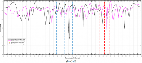
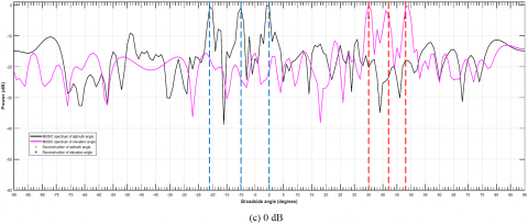
Simulated plots of OMP based reconstruction and $2-\mathrm{D}$ MUSIC by single snapshot of DOA estimation for sparse/dense L-shape array for three sources located at $(\theta, \phi)=\left(35^{0},-21^{0}\right),\left(42^{0},-10^{0}\right)$ and $\left(48^{0}, 0^{0}\right)$ in the far field at various SNRs are shown in Figure $2 .$
The black and the magenta continuum represents the MUSIC spectrum for azimuth and elevation angles respectively for a $N=127$ dense L-shaped array. The peaks are created at the estimated DOAs of the signal. The yellow and the purple asterisks signifies the peak values of the reconstructed power continuum of the proposed reconstruction method of CS-OMP in dB for azimuth and elevation angles respectively for $M=16$ random samples. The vertical blue and red dashed lines indicate the actual DOAs of the target signals in azimuth and elevation angles respectively.
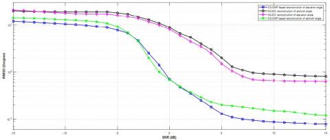
Figure 3 shows the simulated comparison plot of root mean square error (RMSE) of the elevation and azimuth angle estimation with the variation of SNR values between $\pm 15 d B$ with steps of $1 d B$ for both OMP based compressively sensed undetermined reconstruction and MUSIC by using Eq. (18) with $M_{c}=100$ Monte Carlo trials.
Figure 4 shows the simulation of variation of probability of resolution $\left(P_{r e s}\right)$ of the elevation and azimuth angle estimation with the similar variation of SNR values between $\pm 15 d B$ with steps of $1 d B$ for both CS-OMP based undetermined reconstruction and MUSIC by using Eqn. ( $19)$
It is evident from Figure 2 that CS-OMP based underdetermined DOA estimation by single snapshot using sparse L-shaped array over-achieves the standard 2D-MUSIC estimate, particularly at low SNR values. Predominantly, at $\mathrm{SNR}=-15 d B$ and $-5 d B(\text { Figure } 2(a) \text { and }(b))$ the CS-OMP based method completely outclasses MUSIC. As MUSIC looks for eigenvalue decomposition of the array correlation matrix (to exploit the noise eigenvector subspace), at low SNR values the formation of the array correlation matrix nearly becomes deficient. In contrast, the compressive sensing based approach exploits the sparsity character of the impinging signals on the array and efficient recovery suits conceivable using the orthogonal matching pursuit, based on a small number of noisy measurements. As OMP is an iterative greedy algorithm, it selects a column of $\Phi$ at each step which is most correlated with the current residuals. By solving the least square problem a new estimate is calculated provided mutual incoherence exists between $\Phi$ and $\Psi$.
At equivalent and high SNR values also CS-OMP based approach performs better as compared to MUSIC based estimate. The above interpretations turn out to be more apparent if we observe Figure 4. The error (RMSE) committed for elevation and azimuth angle estimation at lower SNR values are much lesser for CS-OMP based approach as compared to MUSIC. At higher SNR values, the error committed for MUSIC decreases, but CS-OMP based reconstruction commits considerable lower estimation errors.
From Figure 3 and Figure 4, it is clear that the proposed method of signal reconstruction by CS-OMP outperforms the standard 2-D MUSIC method, particularly at low SNR values. Also at considerable higher SNR, the error committed and the resolution to resolve the target locations are fared better by CS-OMP method.
In the next simulation, we compute and compare the complexity levels of the standard $2-\mathrm{D} \mathrm{MUSIC}$ and the proposed CS-OMP based reconstruction methods. Table 1 lists the complexity measures. $N$ represents the size of the signal while $K$ is the sparsity level of the signal. $M$ signifies the total number of collected or measured samples such that M>N.
Table 1. Comparison on computational complexity
|
Algorithm |
Complexity |
|
2D-MUSIC |
$\mathcal{O}\left(N^{3}+K N^{2}\right)$ |
|
Proposed CS-OMP |
$\mathcal{O}(K M N)$ |
Table 2 shows the simulation of failure rate of 2-D MUSIC and the proposed CS-OMP based algorithms. The failure rate is measured as the percentage of failed trials in total trials. A trial is said to be succeeded if the estimated signal $\widehat{x}$ is not same as the $K$ largest true indices. From Table $2,$ it is clear the CS-OMP based method has lower failure rate for both azimuth and elevation angles.
Table 2. Comparison of failure rate
|
Algorithm |
Failure Rate |
|
2D-MUSIC |
0.33 |
|
Proposed CS-OMP |
0.09 |
Figure 2. Plot of DOA estimation using 2-D MUSIC and CS-OMP based reconstruction for varying SNR
Figure 3. Plot of variation of RMSE of DOA estimation with SNR
Figure 4. Plot of variation of probability of resolution $\left(P_{r e s}\right)$ of DOA estimation with SNR
Table 3 shows the simulation of execution times of 2-D MUSIC and CS-OMP algorithms for DOA estimation. It is clear that the proposed method requires lesser reconstruction time as compared to standard MUSIC.
Table 3. Comparison of reconstruction time
|
Algorithm |
Reconstruction Time (sec) |
|
2D-MUSIC |
0.053 |
|
Proposed CS-OMP |
0.008124 |
At equivalent and high SNR values also CS-OMP based approach performs better as compared to MUSIC based estimate. The above interpretations turn out to be more apparent if we observe Figure 4. The error (RMSE) committed for elevation and azimuth angle estimation at lower SNR values are much lesser for CS-OMP based approach as compared to MUSIC. At higher SNR values, the error committed for MUSIC decreases, but CS-OMP based reconstruction commits considerable lower estimation errors.
Simulation results of Table 2, 3 and 4 are carried at $S N R=0 d B$, considering equivalent signal and noise power levels.
Decent estimation of the target locations by CS-OMP method at low SNR by single snapshot generate suitable application area in hostile environments, where the signal power is very less as compared to the noise power. This increases the prospect of development of an intelligent, cognitive radar system that can locate and track quasi-stationary objects, including human beings. The L-shaped array, with all its benefits in DOA estimation, together with compressive sensing based OMP reconstruction method can provide information of things or human lives trapped inside a building or behind a wall, to the military or police to take instant decisions. As modern day warfare practises are predominantly bound to urban combat, shrewd enemy or terrorists may deploy jammers and high power interferers to lower the SNR level, thus blocking possible tracking and locating their movements within a building. O'connor et al. [32] provides a good method to mitigate jamming and interferences up to a certain level, but the technique is based on GPS tracking, which may not be feasible always in urban battleground. Thus, CS-OMP based reconstruction method using a sparse L-shaped array structure can be implemented in a synthetic aperture radar (SAR) for through-the-wall-radar imaging (TWRI) applications in unfavourable circumstances.
In a severe multi-path consequence, as in a densely populated mobile communication environment, more accurate DOA estimation or localization of a source mobile station can be achieved in a single snapshot with low complexity by using the CS-OMP based sparse reconstruction approach with a L-shaped array at the base station. Consequently, the SNR is very low in a multi-path scenario with multi-path signals impinging on the receiver array from various directions from the same or different source. The proposed method can be used to identify or localize a source more accurately in a low SNR conditions with lesser complexity.
In this paper, we recommend a method of estimation of 2-D DOA of sources by single snapshot at the far field using an L-shaped array by compressive sensing. Orthogonal Matching Pursuit algorithm is used at the reconstruction. It is a greedy iterative algorithm which is single snapshot based. It requires less number of samples and much lower computationally complex compared to eigen-decomposition, like MUSIC. The failure rate and reconstruction time are also very low. The performance of the proposed method is compared with the standard MUSIC algorithm for 2-D DOA estimation, RMSE and probability of resolution measure. Simulation results show that the proposed method outperforms MUSIC, particularly at low SNR. This becomes more evident from the RMSE and vs SNR (dB) plot. More accurate direction finding with lower complexity and single snapshot is achievable. The proposed method incorporated with the L-shaped array can lead to the development of synthetic aperture radar systems which can be a very effective in hostile situations, like urban warfare scenario. Also, base station antennas can be incorporated with CS-OMP based sparse L-shaped array for multi-path mitigation.
The first author would like to acknowledge the Ministry of Electronics and Information Technology (MeitY), Government of India for supporting and financial assistance during research work through ‘Visvesvaraya Ph.D. Scheme for Electronics and IT’ (Unique Awardee Number: VISPHD-MEITY-1742).
[1] Schmidt, R. (1986). Multiple emitter location and signal parameter estimation. IEEE Transactions on Antennas and Propagation, 34(3): 276-280. http://dx.doi.org/10.1109/TAP.1986.1143830
[2] Roy, R., Paulraj, A., Kailath, T. (1986). Estimation of signal parameters via rotational invariance techniques-ESPRIT. MILCOM 1986, October 1986. http://dx.doi.org/10.1109/MILCOM.1986.4805850
[3] Stoica, P., Sharman, K.C. (1990). Maximum likelihood methods for direction-of-arrival estimation. IEEE Transactions on Acoustics, Speech and Signal Processing, 38(7): 1132-1143. http://dx.doi.org/10.1109/29.57542
[4] Gu, F.J., Zhu, W.P., Swamy, M.S. (2015). Joint 2-D DOA estimation via sparse L-shaped array. IEEE Transactions on Signal Processing, 63(5): 1171-1182. http://dx.doi.org/10.1109/TSP.2015.2389762
[5] Hua, Y., Sarkar, K.T., Wiener, D.D. (1991). An L-shaped array for estimating 2-D directions of arrival. IEEE Transactions on Antennas and Wave Propagation, 39(2): 143-146. http://dx.doi.org/10.1109/8.68174
[6] Ganguly, S., Kerketta, J., Kishore Kumar, P., Mukhopadhyay, M. (2017). A study on DOA estimation algorithms for array processing applications. IEEE-International Conference on Computing and Communication Technologies for Smart Nation (IC3TSN), Gurgaon, New Delhi. http://dx.doi.org/10.1109/IC3TSN.2017.8284451
[7] Zhang, X.F., Li, J.F., Xu, L.Y. (2011). Novel two-dimensional DOA estimation with L-shaped array. EURASIP Journal on Advances in Signal Processing, 50(2011). http://dx.doi.org/10.1186/1687-6180-2011-50
[8] Yan, F.G., Shen, Y., Jin, M. (2015). Fast DOA estimation based on split subspace decomposition on the array covariance matrix. ELSEVIER-Signal Processing, 115: 1-8. http://dx.doi.org/10.1016/j.sigpro.2015.03.008
[9] Lu, G., Hu, B., Zhang, X. (2017). A two-dimensional DOA tracking algorithm using PAST with L-shaped array. Procedia Computer Science, 107: 624-629. https://doi.org/10.1016/j.procs.2017.03.167
[10] Madanayake, A., Wijenayake, C., Wijayaratna, S., Acosta, R., Hariharan, S. I. (2014). 2-D IIR time-delay-sum linear aperature arrays. IEEE Antennas and Wireless Propagation Letters, 13: 591-594. http://dx.doi.org/10.1109/LAWP.2014.2312109
[11] Godara, L.C. (1997). Application of antenna arrays to mobile communications, Part-II: Beamforming and direction-of-arrival considerations. Proceedings of IEEE, 85(8): 1195-1245. http://dx.doi.org/10.1109/5.622504
[12] Porozantzidou, M.G., Chryssomallis, M.T. (2010). Azimuth and elevation angles estimation using 2-D MUSIC algorithm with an L-shaped array. IEEE Antennas and Propagation Society International Symposium. Toronto, ON, Canada. http://dx.doi.org/10.1109/APS.2010.5560953
[13] Gu, J.F., Wei, P. (2007). Joint-SVD of two cross-correlation matrices to achieve automatic pairing in 2-D angle estimation problems. IEEE Antennas and Wave Propagation Letters, 6: 553-556. http://dx.doi.org/10.1109/LAWP.2007.907913
[14] Kikuchi, S., Tsuji, H., Sano, A. (2006). Pair matching method for estimating 2-D angle of arrival with cross-correlation matrix. IEEE Antennas and Wave Propagation Letters, 5: 35-40. http://dx.doi.org/10.1109/LAWP.2005.863610
[15] Tayem, N., Majeed, K., Hussain, A.A. (2016). Two-dimensional DOA estimation using cross-correlation matrix with L-shaped array. IEEE Antennas and Wireless Propagation Letters, 15: 1077-1080. http://dx.doi.org/10.1109/LAWP.2015.2493099
[16] Tayem, N. (2012). Estimation of 2D DOA of coherent signals using a new antenna array configuration. MILCOM 2012, October 2012, Orlando, USA. http://dx.doi.org/10.1109/MILCOM.2012.6415816
[17] Beking, T., Van, M. (2016). Sparse array antenna signal reconstruction using compressive sensing for direction of arrival estimation. Faculty of Electrical Engineering, Mathematics and Computer Science, University of Twente, Master's Thesis. http://purl.utwente.nl/essays/69575
[18] Fortunati, S., Grasso, R., Gini, F., Greco, M.S., LePage, K. (2014). Single snapshot DOA estimation using compressive sensing. IEEE International Conference on Acoustics, Speech and Signal Processing (ICASSP), Florence, Italy. http://dx.doi.org/10.1109/ICASSP.2014.6854009
[19] Candes, E.J., Romberg, J., Tao, T. (2006). Robust uncertainty principles: Exact signal reconstruction from highly incomplete frequency information. IEEE Transactions on Information Theory, 52(2): 489-509. http://dx.doi.org/10.1109/TIT.2005.862083
[20] Hu, Y., Yu, X. (2017). Research on the application of compressive sensing theory in DOA estimation. IEEE International Conference on Signal Processing. Communications and Computing (ICSPCC), Xiamen, China. http://dx.doi.org/10.1109/ICSPCC.2017.8242461
[21] Zhao, L., Xu, J., Ding, J., Liu, A., Li, L. (2017). Direction-of-arrival estimation of multipath signals using independent component analysis and compressive sensing. PloS One, 12(7): e0181838. http://dx.doi.org/10.1371/journal.pone.0181838
[22] Yu, H., Qiu, X., Zhang, X., Wang, C., Yang, G. (2015). Two-dimensional direction of arrival (DOA) estimation for rectangular array via compressive sensing trilinear model. International Journal of Antennas and Propagation, 2015: 10 pages. https://doi.org/10.1155/2015/297572
[23] Zhang, Y., Wan, Q., Yang, W.L. (2007). Solution to linear inverse problem with MMV having linearly varying sparsity structure. 2007 IEEE Radar Conference, April 2007, Boston, USA. http://dx.doi.org/10.1109/RADAR.2007.374287
[24] Cotter, S.F., Rao, B.D., Engan, K., Kreutz-Delgado, K. (2005). Sparse solutions to linear inverse problems with multiple measurement vectors. IEEE Transactions on Signal Processing, 53(7): 2477-2488. http://dx.doi.org/10.1109/TSP.2005.849172
[25] Candes, E., Tao, T. (2005). Decoding by linear programming. IEEE Transactions on Information Theory, 53(12): 4203-4215. http://dx.doi.org/10.1109/TIT.2005.858979
[26] Srinivas, K., Srinivas, N., Kumar, P.K., Pradhan, G. (2018). Performance comparison of measurement matrices in compressive sensing. In International Conference on Advances in Computing and Data Sciences, Springer, Singapore, pp. 342-351. http://dx.doi.org/10.1007/978-981-13-1810-8_34
[27] Ganguly, S., Ghosh, I., Ranjan, R., Ghosh, J., Kumar, P.K., Mukhopadhyay, M. (2019). Compressive sensing based off-grid DOA estimation using OMP algorithm. In 2019 6th International Conference on Signal Processing and Integrated Networks (SPIN), pp. 772-775. http://dx.doi.org/10.1109/SPIN.2019.8711677
[28] Tropp, J.A., Gilbert, A.C. (2007). Signal recovery from random measurements via orthogonal matching pursuit. IEEE Transactions on Information Theory, 53(12): 4655-4666. http://dx.doi.org/10.1109/TIT.2007.909108
[29] Parker, J.T., Cevher, V., Schniter, P. (2011). Compressive sensing under matrix uncertainties: An approximate message passing approach. In 2011 Conference Record of the Forty Fifth Asilomar Conference on Signals, Systems and Computers (ASILOMAR). pp. 804-808. https://doi.org/10.1109/ACSSC.2011.6190118
[30] Rabah, H., Amira, A., Mohanty, B. K., Almaadeed, S., Meher, P.K. (2014). FPGA implementation of orthogonal matching pursuit for compressive sensing reconstruction. IEEE Transactions on very large scale integration (VLSI) Systems, 23(10): 2209-2220. https://doi.org/10.1109/TVLSI.2014.2358716
[31] Van Trees, H.L. (2004). Optimum Array Processing: Part IV of Detection, Estimation, and Modulation Theory. John Wiley & Sons. https://doi.org/10.1002/0471221104
[32] O'connor, A., Setlur, P., Devroye, N. (2015). Single sensor RF emitter localization based on multipath exploitation. IEEE Transactions on Aerospace and Electronic Systems, 51(3): 1635-1651. http://dx.doi.org/10.1109/TAES.2015.120807