Mohammadali Shafieian* | Mohammad Zavar | Mojdeh Rahmanian
© 2019 IIETA. This article is published by IIETA and is licensed under the CC BY 4.0 license (http://creativecommons.org/licenses/by/4.0/).
OPEN ACCESS
The operating range of compressors is usually limited by an unwanted phenomenon that is called, surge. Surge not only limits compressor performance and efficiency, but it can also damage the compressor, such as breaking impellers, oscillation and increasing temperature in compressor. This paper aims to present the application of nonlinear control methods and Lyapunov theory to prevent any surge conditions, in constant speed centrifugal compressors, based on the well-known Moore-Greitzer (MG) model. The only actuator in our system is a close-coupled valve (CCV). We propose a technique for designing nonlinear controllers according Lyapunov Law to avoid surge. In this paper, two controllers are designed and are applied to Moore-Greitzer model for a centrifugal compressor and compared both of them. Simulation results show these controllers can stabilize the instabilities due to surge phenomenon and effectiveness of proposed controllers. The findings of this research may serve as systems that utilizing centrifugal compressors in power generation plants.
centrifugal compressor, surge modeling, nonlinear function, close-coupled valve, Lyapunov, surge protection, control valve, stability
Centrifugal compressors were first invented in the 19th century by Auguste Rateau. Compressors have a wide variety of applications, such as turbo jet engines, turbo charging of internal combustion engines, power generation using industrial gas turbines, pressurization of gas and fluids in the process industry and so on. In general, there are four types of compressors which are reciprocating, rotary, centrifugal and axial [1].
Compression systems such as gas turbines may face with several types of instabilities: combustion instabilities, aero elastic instabilities such as flutter and also aerodynamic flow instabilities. Two types instabilities in aerodynamic flow that can be experienced in compressors are known as surge and rotating stall. Surge is an unwanted flow oscillation through the compressor, and can damage the compressor. It is characterized by a limit cycle in the compressor characteristic [1]. Major damages are breaking impellers, return flow to downstream, oscillation and increasing temperature in compressor.
In many years ago, the solution to this unwanted phenomenon was surge avoidance in which the compressor operating point is never allowed to tend toward the stability limit that is called the surge line. Disadvantage of these techniques is that they have low efficiency and low pressure; therefore, these techniques decrease stable operating range of the compression system [2].
Several methods have been proposed to control surge and can be used to boost efficiency and stabilize the compression system operating range by going closer to the surge line. These Methods are implemented based on either better compressor interior design or variable geometry that can be used for mechanical engineers and methods which control surge by a control law that can be used for automation and control engineers. Therefore, active surge control is more useful than avoiding it [3]. In active control methods, measurements from one or more parameter such as flow and pressure according to a control law, are applied to an actuator so that stability can be achieved in the unstable area of the compressor map [4]. Active control surge has been used since 1989 and many researches about it have been presented [5].
The most powerful techniques are Lyapunov-based controllers based on Greitzer model [6], adaptive control [7], backstepping [8], bifurcation [9], H∞ [10], second-order sliding mode control (2-SM) [11], variable structure [12], fuzzy logic control (FLC) [13] and predictive control based on Lease-Squared Support Vector Machine (LS-SVM) [14, 15].
Several actuators are used for controlling surge. Some of them are closed coupled valve [1], tip clearance [16], bleed valves [17], inlet guide vanes [18], recirculation [19], air injection [20] and Throttle Control Valve [21]. But the most famous actuators which have been used recently are closed coupled valve and Throttle Control Valve. In past researches one or both of them have been used. Although designing two controllers for two actuators is difficult, but it is used.
This paper represents the application of nonlinear active control for surge control in constant speed centrifugal compressors according to the famous Moore-Greitzer (MG) model according to Lyapunov control law. In most past researches, two control valves are used which called CCV (closed couple valve) and TCV (throttle control valve) to avoid unwanted surge phenomenon; but in this paper, Surge is controlled with only CCV. The scientific contributions of this paper are simplicity of designing and setting up one controller instead of two controllers (old methods) and good efficiency and performance of compressor. Two controllers are presented and compared. Results show that the first controller has better efficiency.
The remainder of the paper is organized as follows. In section 2, we introduce the model of the system and mathematical equations for Moore-Greitzer model. In section 3, we formulate the first controller. In section 4, we present its simulation results. In sections 5, model and problem formulation of the second controller are introduced. Section 6, includes Simulation results of the second controller. This is followed by conclusions in section 7.
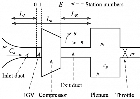
Although several dynamic models for the unstable operation behavior of compression systems have been presented since 1955, we refer to the famous nonlinear compressor model suggested by Moore and Greitzer. This model is shown in Figure 1.
Figure 1. Compression system, Figure taken from Moore and Greitzer [1]
According to Simon and Valavani [20], close-coupled control valve (CCV) is in series with compressor and we can assume that no considerable mass storage can occur since the distance between the compressor outlet and CCV is so small. After CCV there is a plenum volume for storage compressible gas. It is shown in Figure 2.
Figure 2. Compression system with CCV [1]
The two differential equations of the model Moore-Greitzer is given by:
$\dot{\Psi}=\frac{1}{4 B^{2} L_{c}}\left(\Phi-\Phi_{T}(\Psi)\right)$ (1)
$\dot{\Phi}=\frac{1}{L_{C}}\left(\Psi_{C}(\Phi)-\Psi\right)$ (2)
in which, B is Greitzer parameter, Lc is Length of compressor and Duct, Φ is averaged mass flow coefficient and is given by:
$\Phi=\frac{c_{x}}{U}$ (3)
where, Cx is axial velocity and U is blade speed. And:
$\dot{\Psi}=\frac{d \Psi}{d \xi}$ (4)
$\dot{\Phi}=\frac{d \Phi}{d \xi}$ (5)
$\xi$ is nondimensional time and is defined as:
$\xi=\frac{U t}{R}$ (6)
where, R is the mean compressor radius. Furthermore, Ψ is pressure coefficient and is given by:
$\psi=\frac{P_{1}-P_{o 1}}{\rho U^{2}}$ (7)
in which, P1 is output pressure coefficient of the compressor, Po1 is input pressure coefficient of the compressor and ρ is density.
On the other hand, $\Phi_{T}(\Psi)$ is throttle mass flow coefficient and is expressed by $\Phi_{T}(\Psi)=\gamma_{T} \sqrt{\Psi},$ in which $\gamma_{T}$ is throttle gain valve. $\Psi_{C}(\Phi)$ is pressure rise in the compressor and is a nonlinear function of the mass flow (compressor characteristic). $\Psi_{C}(\Phi)$ can be formulated as:
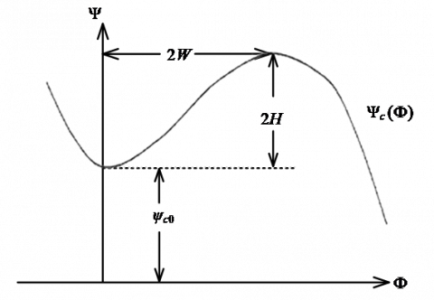
$\Psi_{c}(\Phi)=\Psi_{\mathrm{C} 0}+\mathrm{H}\left(1+\frac{3}{2}\left(\frac{\Phi}{\mathrm{w}}-1\right)-\frac{1}{2}\left(\frac{\Phi}{\mathrm{w}}-1\right)^{3}\right)$ (8)
in which ΨC0 is constant shut-off value of the compressor characteristic, H is semi Height and W is semi width, as shown in Figure 3.
Figure 3. Cubic compressor characteristic of Moor-Greitzer [1]
Table 1. Numerical values for a typical compressor
|
B=1.8 |
$\psi_{c 0}=0.3$ |
|
$\rho=1.15 \frac{\mathrm{kg}}{\mathrm{m}^{3}}$ |
$\gamma_{T}=0.61$ |
|
H=0.18 |
$L_{c}=3 m$ |
|
$\Phi_{0}=0.6$ |
w=0.25 |
$\widehat{\Psi}=\Psi-\Psi_{0}$ (9)
$\widehat{\Phi}=\Phi-\Phi_{0}$ (10)
so, $\widehat{\Psi}_{C}(\widehat{\Phi})$ is defined as:
$\widehat{\Psi}_{C}(\widehat{\Phi})=\psi_{C}\left(\widehat{\Phi}+\Phi_{0}\right)-\Psi_{0}$ (11)
by substituting (3) in (7), we have:
$\widehat{\Psi}_{C}(\widehat{\Phi})=\Psi_{\mathrm{C0}}-\Psi_{0}-\frac{\mathrm{H}}{2 \mathrm{W}^{3}} \widehat{\Phi}^{3}-\frac{3 \mathrm{H}}{2 \mathrm{W}^{2}}\left(\frac{\Phi_{0}}{\mathrm{W}}-1\right) \widehat{\Phi}^{2}-\frac{3 \mathrm{H} \Phi_{0}}{2 \mathrm{W}^{2}}\left(\frac{\Phi_{0}}{\mathrm{w}}-2\right) \widehat{\Phi}-\frac{\mathrm{H} \Phi_{0}^{2}}{2 \mathrm{W}^{2}}\left(\frac{\Phi_{0}}{\mathrm{w}}-3\right)$ (12)
$\widehat{\Psi}_{C}(\widehat{\Phi})=-K_{3} \widehat{\Phi}^{3}-K_{2} \widehat{\Phi}^{2}-K_{1} \widehat{\Phi}+\widehat{\Psi}_{\mathrm{CO}}$ (13)
in which,
$K_{3}=\frac{\mathrm{H}}{2 \mathrm{W}^{3}}$ (14)
$K_{2}=\frac{3 \mathrm{H}}{2 \mathrm{W}^{2}}\left(\frac{\Phi_{0}}{\mathrm{w}}-1\right)$ (15)
$K_{1}=\frac{3 \mathrm{H} \Phi_{0}}{2 \mathrm{W}^{2}}\left(\frac{\Phi_{0}}{\mathrm{W}}-2\right)$ (16)
$\widehat{\mathrm{H}}_{\mathrm{CO}}=\mathrm{H}_{\mathrm{CO}}^{\mathrm{J}}-\Psi_{0}-\frac{\mathrm{H} \Phi_{0}^{2}}{2 \mathrm{W}^{2}}\left(\frac{\Phi_{0}}{\mathrm{w}}-3\right)$ (17)
According to Table 1, $\widehat{\Psi}_{\mathrm{C0}}$ is very small and assumed to be zero for simplicity. Therefore, (1) and (2) are converted to (18) and (19).
$\dot{\hat{\psi}}=\frac{1}{4 B^{2} L_{c}}\left(\widehat{\Phi}-\widehat{\Phi}_{T}(\hat{\psi})\right)$ (18)
$\dot{\widehat{\Phi}}=\frac{1}{L_{c}}\left(\hat{\psi}_{c}(\widehat{\Phi})-\hat{\psi}\right)$ (19)
In this section, the first controller will be designed for the pure surge case. In [20], Simon and Valavani recommended using the drop in pressure across the valve as the control variable u. we use that idea for operating compressor close the surge line without any oscillation. In case of pure surge, the model is given by:
$\dot{\hat{\psi}}=\frac{1}{4 B^{2} L_{c}}\left(\widehat{\Phi}-\widehat{\Phi}_{T}(\hat{\psi})\right)$ (20)
$\dot{\widehat{\Phi}}=\frac{1}{L_{c}}\left(\hat{\psi}_{c}(\widehat{\Phi})-u-\hat{\psi}\right)$ (21)
The assumed controller can be formulated as:
$u=C \widehat{\Phi}^{2}=C\left(\Phi-\Phi_{0}\right)^{2}$ (22)
where, C is a constant value (gain of controller) and will be calculated in the following. The control Lyapunov function (CLF) for this step is selected as:
$V(\hat{\psi}, \widehat{\Phi})=\hat{\psi}^{2}+\widehat{\Phi}^{2}$ (23)
For simplicity and eliminating constant coefficients, it is modified as [1]:
$V(\hat{\psi}, \widehat{\Phi})=2 B^{2} L_{C} \hat{\psi}^{2}+\frac{L_{C}}{2} \widehat{\Phi}^{2}$ (24)
Based on laws for stability of control Lyapunov function, $\dot{V}$ which is the first order derivate of Lyapunov function, must be negative, so we have:
$\dot{V}=4 B^{2} L_{C} \hat{\psi} \dot{\hat{\psi}}+L_{C} \widehat{\Phi} \dot{\hat{\Phi}}$ (25)
By substituting (20)-(21) in (25), we have:
$\dot{V}=\hat{\psi} \widehat{\Phi}-\hat{\psi} \widehat{\Phi}_{T}(\hat{\psi})+\widehat{\Phi} \hat{\psi}_{c}(\widehat{\Phi})-C \widehat{\Phi}^{3}-\hat{\psi} \widehat{\Phi}<0$ (26)
Throttle valve is passive, and then $\widehat{\boldsymbol{\Phi}}_{T}(\widehat{\psi})$ is always positive; therefore $-\widehat{\psi} \widehat{\boldsymbol{\phi}}_{T}(\widehat{\psi})<0 ;$ So:
$\widehat{\Phi} \hat{\psi}_{c}(\widehat{\Phi})-C \widehat{\Phi}^{3}<0$ (27)
By substituting (13) in (27), we have:
$-K_{3} \widehat{\Phi}^{4}-K_{2} \widehat{\Phi}^{3}-K_{1} \widehat{\Phi}^{2}--C \widehat{\Phi}^{3}<0=-K_{3} \widehat{\Phi}^{2}\left[\widehat{\Phi}^{2}+\frac{K_{2}}{K_{3}} \widehat{\Phi}+\frac{K_{1}}{K_{3}}+\frac{C}{K_{3}} \widehat{\Phi}\right]<0$ (28)
By using the numerical values of Table $2,$ we conclude that $K_{3}>0 .$ Thus $-K_{3} \widehat{\Phi}^{2}<0 .$ It's enough to show:
$\left[\widehat{\Phi}^{2}+\frac{K_{2}}{K_{3}} \widehat{\Phi}+\frac{K_{1}}{K_{3}}+\frac{C}{K_{3}} \widehat{\Phi}\right]<0$ (29)
It is easy to show that it’s necessary:
$C<2 \sqrt{K_{1} K_{3}}-K_{2}$ (30)
By using the numerical values of Table 1, the values of Table 2 are achieved.
Table 2. Numerical values for the first controller
|
K1=1.036 |
K3=5.76 |
|
C<-1.16 |
K2=6.048 |
According to the values, obtained in previous chapter, we apply the controller to Moore-Greitzer model. We assume C=-2 thus we expect the system to be stable. Simulation Results are shown in Figure 4-6.
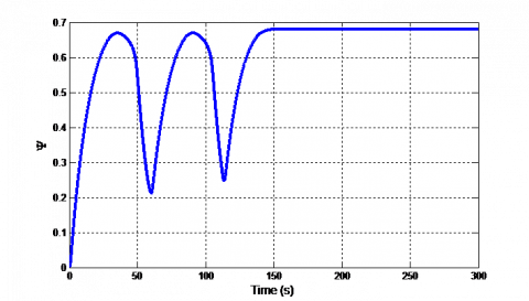
It can be seen from Figure 4 that there is no controller and the compressor is in surge position, at first. By applying the controller at nearly t=110 s the compressor mass flow increases, and then by eliminating the surge, the compressor mass flow stabilizes. This stability is achieved at equilibrium point approximately.
Figure 4 shows that initially there is no controller and the compressor is in surge position. By applying the controller at nearly t=110 s the mass flow increases, and so by eliminating the surge, the mass flow at the output stabilizes. This stability is also achieved at equilibrium point approximately.
Figure 4. Compressor mass flow coefficient when C=-2 and applying controller at t=110s
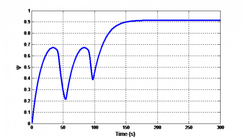
Figure 5. Compressor pressure coefficient when C=-2 and applying controller at t=120s
Figure 5 shows that initially there is no controller and the compressor is in surge position. By applying the controller at nearly t=120 s the pressure increases, and so by eliminating the surge, the pressure at the output stabilizes. This stability is also achieved at equilibrium point approximately.
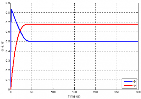
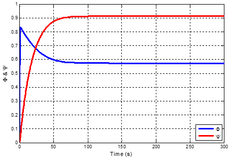
Figure 6. Compressor mass flow and pressure coefficient when C=-2 and always applying controller
Figure 6 shows that initially there is controller so the compressor operates stability at equilibrium point approximately
In this chapter, another law is considered for the controller, u. The control law can be stated as:
$u=C_{1} \widehat{\Phi}+C_{2} \dot{\vec{\Phi}}+\frac{c_{2}}{L_{C}} \widehat{\Psi}$ (31)
By substituting $(1)-(2)$ in $(31)$ , we have:
$u=\frac{c_{1} L_{C} \hat{\Phi}+C_{2} \hat{\Psi}_{C}(\hat{\Phi})}{C_{2}+L_{C}}$ (32)
Here the control Lyapunov function for this step is determined as same as (24). Similar to chapter 3, by substituting (20), (21) and (32) in (25) and by applying laws for stability of control Lyapunov function, we have:
$\dot{V}=-\widehat{\psi} \widehat{\Phi}_{T}(\widehat{\psi})+\widehat{\Phi} \widehat{\psi}_{c}(\widehat{\Phi})-\frac{c_{1} L_{c} \widehat{\Phi}^{2}+C_{2} \vec{\Phi} \tilde{\psi}_{c}(\vec{\Phi})}{C_{2}+L_{C}}$ (33)
We assume $C_{2}=1$ and by using the numerical values of Table 1 , we have:
$\dot{V}=-\widehat{\psi} \widehat{\Phi}_{T}(\widehat{\psi})+\frac{1}{2} \widehat{\Phi} \widehat{\psi}_{c}(\widehat{\Phi})-\frac{c_{1}}{2} \widehat{\Phi}^{2}<0$ (34)
Throttle valve is passive, then $\widehat{\Phi}_{T}(\widehat{\psi})$ is always positive. therefore $-\hat{\psi} \widehat{\Phi}_{T}(\hat{\psi})<0 ;$ It's enough that:
$\frac{1}{2} \widehat{\Phi} \widehat{\psi}_{c}(\widehat{\Phi})-\frac{c_{1}}{2} \widehat{\Phi}^{2}<0$ (35)
By substituting (13) in (35), we have:
$\frac{1}{2}\left[-K_{3} \widehat{\Phi}^{4}-K_{2} \widehat{\Phi}^{3}-K_{1} \widehat{\Phi}^{2}-C_{1} \widehat{\Phi}^{2}\right]<0=-\frac{K_{3}}{2} \widehat{\Phi}^{2}\left[\widehat{\Phi}^{2}+\frac{K_{2}}{K_{3}} \widehat{\Phi}+\frac{C_{1}+K_{1}}{K_{3}}\right]<0$ (36)
By using the numerical values of Table 2, we have:
$K_{3}>0$ Therefore $-\frac{K_{3}}{2} \widehat{\Phi}^{2}<0$
It's enough that $\left[\widehat{\Phi}^{2}+\frac{K_{2}}{K_{3}} \widehat{\Phi}+\frac{c_{1}+K_{1}}{K_{3}}\right]<0$ (37)
with (37) It is easy to show that it’s necessary:
$\frac{K_{2}^{2}}{K_{3}^{2}}-4 \frac{C_{1}+K_{1}}{K_{3}}<0$ (38)
By using the numerical the values of Table 2, we have:
$C_{1}>0.55$ (39)
According to the values, obtained in previous chapter, we apply the controller to Moore-Greitzer model. We assume that C1=0.6 thus we expect the system to be stable. Simulation Results are shown in Figure 7-9.
Figure 7. Compressor mass flow coefficient when C1=0.6 and applying controller at t=100s
It can be seen from Figure 7 that there is no controller and the compressor is in surge, at first. By applying the controller at nearly t=100 s the compressor mass flow increases, and then by eliminating the surge, the compressor mass flow stabilizes. This stability is achieved at equilibrium point approximately.
Figure 8. Compressor pressure coefficient when C1=0.6 and applying controller at t=120s
Figure 8 shows that initially there is no controller and the compressor is in surge. By applying the controller at nearly t=120 s the pressure increases, and so by eliminating the surge, the pressure at the output stabilizes. This stability is also achieved at equilibrium point approximately.
Figure 9. Compressor mass flow and pressure coefficient when C1=0.6 and always applying controller
Figure 9 shows that initially there is controller so the compressor operates stability at equilibrium point approximately.
In this paper, a centrifugal compression system which is equipped with CCV has been investigated. Two controllers base on Lyapunov control law are developed for surge suppression. Simulations results show that both of them can stabilize the surge phenomenon and control surge by applying CCV and only one controller.in addition, simulation results as same the results of recent past researches; But the advantages of this results in simplicity of designing and setting up one controller instead of two controllers (old methods) and good efficiency and performance of compressor. Two controllers are presented and compared. The first controller has better performance and more efficiency. Although the second controller has more pressure coefficient, but mass flow coefficient has increased. It yields to less efficiency for the second controller than the first controller. Other methods can be utilized to improve performance of the controller such as using artificial neural networks as a part of controller which will be investigated in our future work.
[1] Gravdahl, J.T., Egeland, O. (2011). Compressor surge and rotating stall: Modeling and control. Springer Publishing Company, Incorporated. https://doi.org/10.1007/978-1-4471-0827-6
[2] Gravdahl, J.T., Willems, F., Jager, B.D., Egeland, O. (2000). Modeling for surge control of centrifugal compresssors: Comparison with experiment. Proceedings of the 39th IEEE Conference on Decision and Control, Sydney, NSW, Australia. https://doi.org/10.1109/CDC. 2000.912043
[3] Shehata, R.S., Abdullah, H.A., Areed, F.F.G. (2008). Fuzzy logic surge control in constant speed centrifugal compressors. 2008 Canadian Conference on Electrical and Computer Engineering, Niagara Falls, ON, Canada. https://doi.org/10.1109/CCECE.2008.4564616
[4] Ma, X., Zheng, S., Wang, K. (2019). Active surge control for magnetically suspended centrifugal compressors using a variable equilibrium point approach. IEEE Transactions on Industrial Electronics, 66(12): 9383-9393. https://doi.org/10.1109/TIE.2019.2891412
[5] Epstein, A.H., Ffowcs Williams, J.E., Greitzer, E.M. (1989). Active suppression of aerodynamic instabilities in turbomachines. Journal of Propulsion and Power, 5(2): 204-211. https://doi.org/10.2514/3.23137
[6] Simon, J.S., Valavani, L. (1991). A lyapunov based nonlinear control scheme for stabilizing a basic compression system using a close-coupled control valve. 1991 American Control Conference, Boston, MA, USA. http://dx.doi.org/10.23919/ACC.1991.4791832
[7] Billoud, G., Galland, M.A., Huynh, C.H., Candel, S. (1991). Adaptive active control of instabilities. Journal of Intelligent Material Systems and Structures, 2(4): 457-471. https://doi.org/10.1177%2F1045389X9100200402
[8] Krstic, M., Protz, J.M., Paduano, J.D., Kokotovic, P.V. (1995). Backstepping designs for jet engine stall and surge control. Proceedings of 1995 34th IEEE Conference on Decision and Control, New Orleans, LA, USA, USA. https://doi.org/10.1109/CDC.1995.478612
[9] Liaw, D.C., Abed, E.H. (1996). Active control of compressor stall inception: A bifurcation-theoretic approach. Automatica, 32(1): 109-115. https://doi.org/10.1016/0005-1098(95)00096-8
[10] Weigl, H.J., Paduano, J.D., Bright, M.M. (1997). Application of H/sub /spl infin// control with eigenvalue perturbations to stabilize a transonic compressor. In Proceedings of the 1997 IEEE International Conference on Control Applications, Hartford, CT, USA. https://doi.org/10.1109/CCA.1997.627739
[11] Bartolini, G., Muntoni, A., Pisano, A., Usai, E. (2008). Compressor surge active control via throttle and CCV actuators. A second-order sliding-mode approach. 2008 International Workshop on Variable Structure Systems, Antalya, Turkey. http://dx.doi.org/10.1109/VSS.2008. 4570720
[12] Shehata, R.S., Abdullah, H.A., Areed, F.F.G. (2009). Variable structure surge control for constant speed centrifugal compressors. Control Engineering Practice, 17(7): 815-833. https://doi.org/10.1016/j.conengprac.2009.02.002
[13] Laderman, M., Greatrix, D., Liu, G. (2003). Fuzzy logic control of surge in a jet engine model. The 13th propulsion symposium, 50th CASI annual conference, Montreal.
[14] Torrisi, G., Grammatico, S., Cortinovis, A., Mercangöz, M., Morari, M., Smith, R.S. (2017). Model predictive approaches for active surge control in centrifugal compressors. IEEE Transactions on Control Systems Technology, 25(6): 1947-1960. https://doi.org/10.1109/TCST.2016.2636027
[15] Wang, C.X., Shao, C., Han, Y. (2010). Centrifugal compressor surge control using nonlinear model predictive control based on LS-SVM. 2010 3rd International Symposium on Systems and Control in Aeronautics and Astronautics, Harbin, China. https://doi.org/10.1109/ISSCAA.2010.5633206
[16] Sanadgol, D., Maslen, E. (2005). Effects of actuator dynamics in active control of surge with magnetic thrust bearing actuation. Proceedings, 2005 IEEE/ASME International Conference on Advanced Intelligent Mechatronics, Monterey, CA, USA. https://doi.org/10.1109/AIM.2005.1511155
[17] Fontaine, D., Shengfang, L., Paduano, J., Kokotovic, P.V. (2004). Nonlinear control experiments on an axial flow compressor. IEEE Transactions on Control Systems Technology, 12(5): 683-693. https://doi.org/10.1109/TCST.2004.826967
[18] Camp, T.R., Day, I.J. (1998). A study of spike and modal stall phenomena in a low-speed axial compressor. Journal of Turbomachinery, 120(3): 393-401. https://doi.org/10.1115/1.2841730
[19] Balchen, J.G., Mumme, K.I. (1987). Process control: Structures and applications. VanNostrand and Reinhold Company, 640.
[20] Behnken, R.L., Murray, R.M. (1997). Combined air injection control of rotating stall and bleed valve control of surge. Proceedings of the 1997 American Control Conference, Albuquerque, NM, USA. https://doi.org/10.1109/ACC.1997.609674
[21] Willems, F., Heemels, W.P.M.H., de Jager, B., Stoorvogel, A.A. (2002). Positive feedback stabilization of centrifugal compressor surge. Automatica, 38(2): 311-318. https://doi.org/10.1016/S0005-1098(01)00202-3